Hydrodynamics

1 Theory

1.1 Star Formation

1.1.1 Jeans instability and mass

The Jeans criteria defines when a gas cloud starts to collapse under its gravitational potential. Therefore we need to take the virial theorem into account: \[2E_{kin} = -E_{pot}\qquad{(1)}\]

The virial theorem is applicable if the gas is in equilibrium: If \(E_{kin}\) is smaller than \(-\dfrac{E_{pot}}{2}\) the gas is not stable and a collapse is possible.

In the case of a cloud with uniform density, the thermal energy \(E_{kin} = \dfrac{3kT}{2\mu m_{u}}M\) and the gravitational potential \(E_{pot} = -\dfrac{3 GM^2}{5R}\) yield:

\[\dfrac{3kT}{\mu m_{u}}M = \dfrac{3 GM^2}{5R}\qquad{(2)}\]

\[\Rightarrow \dfrac{2E_{kin}}{-E_{pot}} = \dfrac{5 kTR}{ GM\mu m_{u}} = 1\qquad{(3)}\]

G: gravitational constant

k: Boltzmann’s constant

\(m_{u}\) : atomic mass unit

\(\mu\): molecular weight of the hole gas

The cloud is going to collapse if its radius is smaller than the Jeans radius

\[R_{J} = \dfrac{GM\mu m_{u}}{5 kT}\qquad{(4)}\]

If we take into account that \(M = \frac{4}{3} \pi \rho R^3\) we can form the Jeans mass. Clouds with temperature T, density \(\rho\), and a mass greater than the Jeans mass are probably not stable.

\[M_{J} = 5.46 \left( \frac{kT}{G\mu m_{u}} \right)^{\frac{3}{2}} \rho^{-\frac{1}{2}}\qquad{(5)}\]

1.1.2 Starforming regions

It follows from the Jeans criteria, that only very large masses can collapse. For a typical density of a molecular cloud (\(10^{-21}\) and \(10^{-18} \frac{kg}{m^3}\)) the Jeans mass is around \(10^5\) to \(10^2 M_{\odot}\). These blobs usually form accretion discs in which the gas is further compressed, so the Jeans mass is reduced to \(10^{-1}\) to \(10^2 M_\odot\). Therefore, large molecular clouds are not always gravitationally bound or unstable. In addition to that molecular clouds have a complex and turbulent substructure, leading to local compressions. Those are called protostellar cores and they have a typical density of around \(10^{-17}\) to \(10^{-15} \frac{kg}{m^3}\). At a temperature around 10K the Jeans mass is \(10^{-1}\) to \(10^2 M_\odot\). Dense protostellar cores can be Jeans unstable and can collapse, which leads to star formation. For non-vanishing angular momentum, the protostellar core forms an accretion disk around the young star which in turn adds even more mass to the central protostar. In some cases the accretion disk is also unstable and able to fragment, forming a multiple star system  [1].

1.1.3 Accretion disk

A gravitationally unstable gas cloud with non-zero angular momentum collapses to an accretion disk. The total angular momentum ensures that on average collisions parallel to the spin axis deaccelerate the particles more than those perpendicular to the spin axis. This leads finally to the formation of an accretion disk. These discs usually don’t rotate as a rigid body, however, with a differential velocity. This results in shear forces transporting the material from the outside to the central star. In some cases these discs fulfill a Kepler motion \(v = \sqrt{\dfrac{GM}{R}}\) and are called Keplerian discs. The mass of the disk can be a hundred times larger than the central star. While the particles move inwards, the angular momentum must be removed to the outside. Due to the viscosity, the angular momentum is transferred to another particle, moving it away from the center.

These accretion discs can become unstable and fragment. In this case, additional protostars are formed and either bound to a multiple star system or kicked out. One criterion for the stability of a disk is the Toomre Q-value.

\[Q = \frac{\sigma_{R} \chi}{3.36 G \sum}\qquad{(6)}\]

With \(\sigma_{R}\) the radial component of the velocity, \(\chi\) the epi-cyclic frequency, and the surface density \(\sum\). If the Toomre Q-value is locally smaller than 1, the disk is unstable at that point and able to collapse.

1.1.4 Protostars

A protostar is a more dense core within a collapsing molecular cloud. A first core is formed after a timescale comparable to the free-fall time \(t_{ff}\). This core usually has less than one percent of the mass of the molecular cloud. More and more mass is continuously falling onto the core, increasing the core’s temperature. If the core has become so dense that it is optically thick, and thus cannot carry away any more heat by radiation, the core further contracts slowly. The surrounding gas continuously falls onto the hot core and it is compressed even further until the H\(_2\) dissociates at a density around \(\rho = 10^{-6} \frac{kg}{m^3}\). The core loses its hydrostatic equilibrium and collapses a second time. The resulting smaller core has a mass around thousands of the primary molecular cloud and a density between 1 to 10 \(\frac{kg}{m^3}\). If the first shell is completely fallen onto the inner core it is called a protostar. In this phase, nearly the whole luminosity is caused by the falling particles’ kinetic energy.

\[L_{acc} \propto \dot{M}_{Core}G\dfrac{M_{Core}}{R_{Core}}\qquad{(7)}\]

With \(\dot{M}_{Core}\) the rate of the in falling particle.

During this process, the rate of infalling particles declines. If the accretion luminosity is negligibly small compared to the comprehension luminosity, the protostar is called a pre-main-sequence star.

1.1.5 Pre-main-sequence star

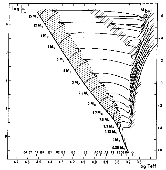
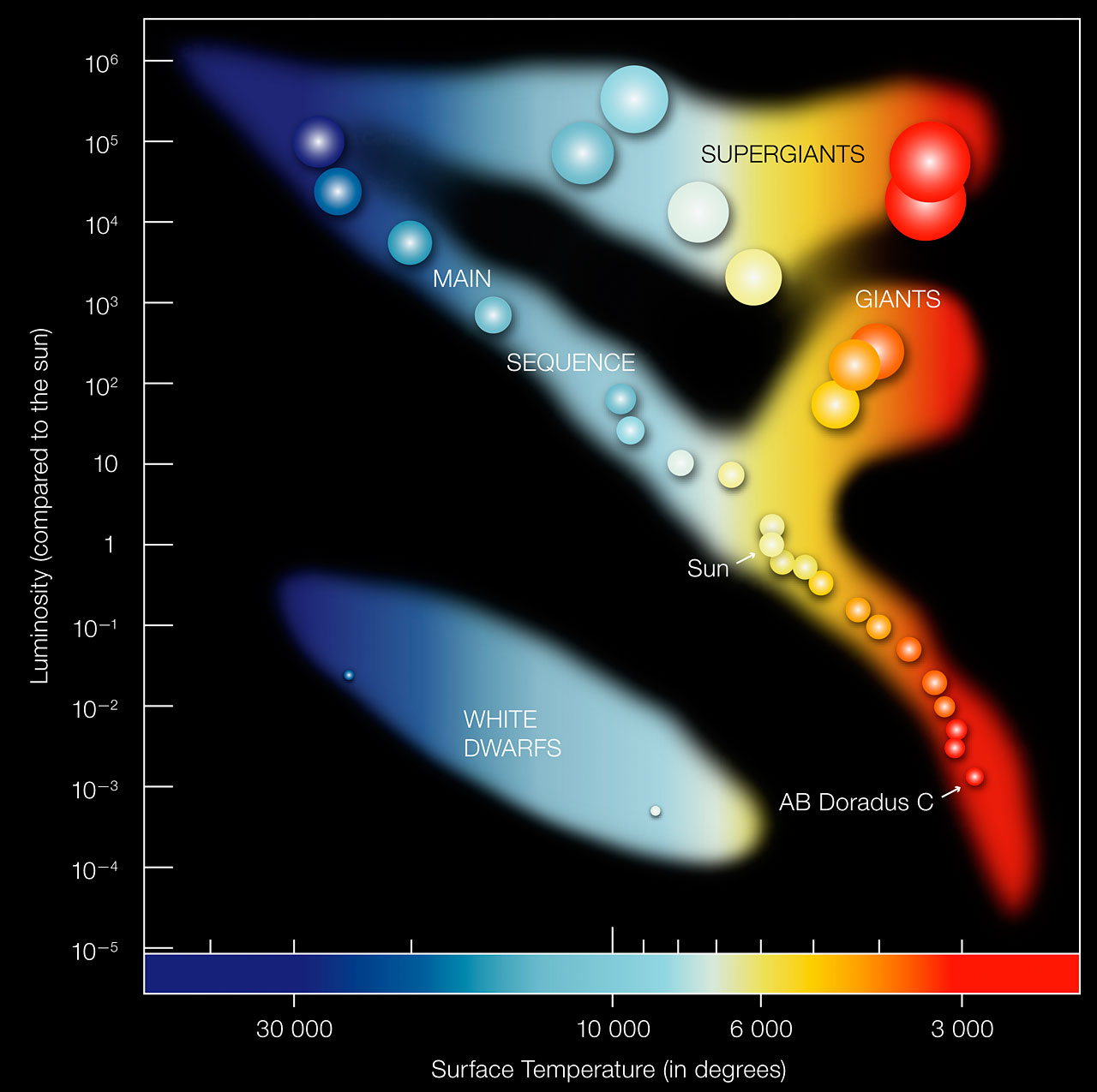
Pre-main-sequence stars are in hydrostatic equilibrium. In the beginning, they have gravitational energy as an energy source. After the protostellar phase, the star is optically visible for the first time. Because protostars are very luminous and cold they are in the upper right corner of the Hertzsprung-Russel-diagram (1). In the Hertzsprung-Russell-diagram the luminosity of a star is plotted against the temperature or the color of a star. While the Pre-main-sequence star contracts it moves along the Hayashi line, which separates the stable (left) from the unstable stars (right)(2). For example, a star with 1 M\(_{\odot}\) starts increasing its temperature after around \(10^7\) years; this leads to a horizontal line in the Hertzsprung-Russell-diagram. Shortly before reaching the main sequence the nuclear fusion starts and stabilizes the star that it stays there for a long time period. Stars with larger masses than 3 M\(_{\odot}\) skip the pre-main-sequence phase and already start nuclear fusion within the protostellar phase.

1.2 Initial mass function (IMF)

The initial mass function (IMF) is an empirical function that sets the frequency of new stars with their masses in context. The IMF \(\phi(M)\) indicates how many stars are located in the mass interval between \((M, M+\Delta M)\). \(\phi(M)\) is normalized as \(\int_{M_{min}}^{M_{max}} \phi(M) M dM = 1\) and the amount of stars within the mass interval dm results in

\[N dM = \phi(M) dM.\qquad{(8)}\]

Edwin Salpeter firstly plotted and fitted observations of stars between \(M=0.5M_{\odot}\) and \(M=10M_{\odot}\) with the relationship \[\phi(M) dM = C M^{-2.35} dM.\qquad{(9)}\]

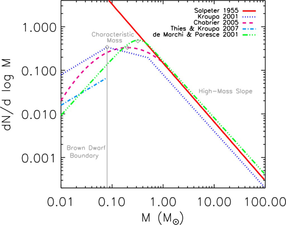
Applying the relationship shown above for very small masses the stellar mass would be dominated by low-mass stars. Recent observations of the IMF, e.g.  [3] and  [4], show that the the IMF’s course for low-mass stars is bent (figure [IMF]). However, there are much more low-mass stars than high-mass stars. The abundance of stars with masses larger than \(M=0.1{M}_{\odot}\) decreases rapidly.

Actual studies fit the IMF for example with  [5]

\[\phi(M) dM = \left\{ \begin{array}{c} C M^{-1.2} - 0.1 {M}_{\odot} < M < 1.0 {M}_{\odot} \\ C M^{-2.7} - 1.0{M}_{\odot} < M < 10 {M}_{\odot} \\ 0.4 C M^{-2.3} - 10 {M}_{\odot} < M \end{array} \right.\qquad{(10)}\]

An alternative description is the log-normal distribution by Miller and Scalo’s:

\[\phi(\log(M)) = A_{0} + A_{1} \log{M} + A_{2} \log(M)^2\qquad{(11)}\]

One of the IMF’s peculiarities is that it (at least in areas for not very low-mass stars) appears approximately equal for all star-formation regions in the Milky Way. However, it is not yet fully understood.

1.3 Model of the isothermal sphere by Shu

A spherically symmetrical cloud with a density profile of \(r^{-2}\) serves as a simple model for star formation. The disadvantage of this model is that it is not stable and therefore physically not very reasonable. The advantage on the other hand is, that it is the only model of a star-forming region with an analytical solution, which makes it possible to compare the results.

It is possible to solve this problem by using Eulerian equations of hydrodynamic for a spheric symmetrical flow.

\[\dfrac{\partial M}{\partial t} + u\frac{\partial M}{\partial r} = 0, \\ \\ \dfrac{\partial M}{\partial r} = 4 \pi r^2 \rho\qquad{(12)}\]

We are looking for self-similar solutions, i.e. solutions that apply to all scales. For this purpose, a dimensionless variable is introduced.

\[x = \frac{r}{at}\qquad{(13)}\]

If there are self-similar solutions they have the form:

\[\rho(r,t) = \frac{\alpha(x)}{4\pi G^2}\qquad{(14)}\] \[M(r,t) = \frac{a^3t}{G}m(x)\qquad{(15)}\] \[u(r,t) = av(x)\qquad{(16)}\] These equations must be solved numerically for \(\rho\)(r,t), M(r,t) and u(r,t).

One possible solution is \[\rho(x,t) = \left(g(x)^{\frac{7}{2}} + h(x)^{\frac{7}{2}} \right)^{\frac{2}{7}}\qquad{(17)}\] \[u(x,t) = \left(g(x)^{\frac{5}{9}} -2^{\frac{5}{9}} \right)^{\frac{9}{10}}\qquad{(18)}\] \[m(x,t) = 1,025x^2+0,975+0.075x(1-x)\qquad{(19)}\] with \[g(x,t) = \dfrac{1}{1.43 x^{\frac{3}{2}}}\qquad{(20)}\] and \[h(x,t) = \frac{2}{x}\qquad{(21)}\]

A shock front forms and moves at supersonic speed from the inside outwards. Inside the shock front, the gas falls in free fall to the center.

This results in a constant accretion rate of the protostar at the center.

\[\dot{M} = 0.975 \frac{c_s^3}{G}\qquad{(22)}\]

The accretion rate is also to be determined in the following experiment and should be compared with the analytical solution of Shu.

2 Smoothed Particle Hydrodynamics

For the following simulations of star formation regions Daniel J. Prices Phantom SPH (Smoothed Particle Hydrodynamics) code is used which is explained in detail in the following section  [6].

2.1 Smoothing of physical properties

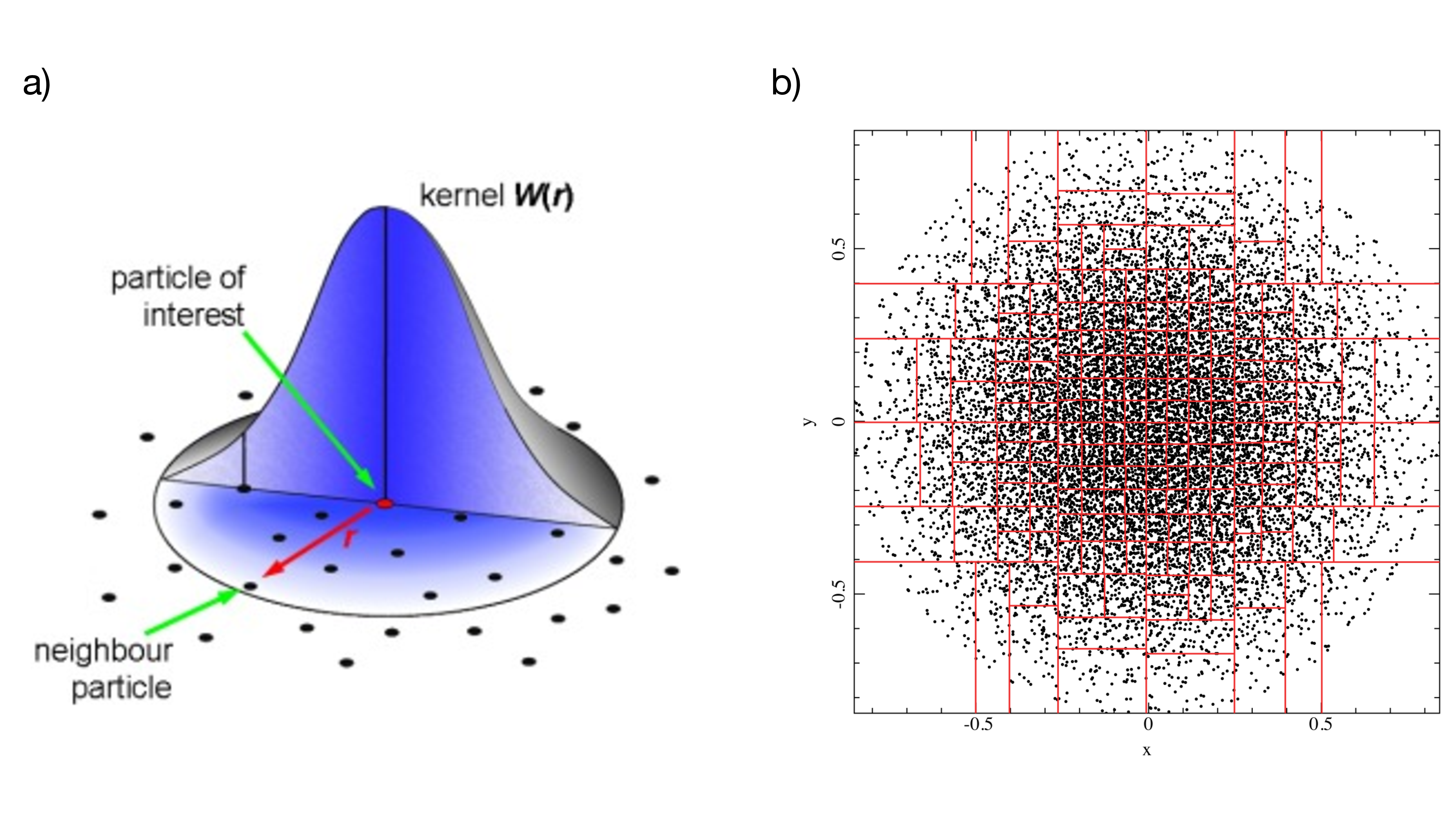
In this kind of simulation the gas is represented as single particles and not, as in other methods, by a lattice. As the name suggests the physical properties of all particles are smoothed. This is done using a weighting function, \(W(r,h)\), often referred to as kernel. \(2h\) is the length throughout the properties are smoothed. The weighting function is similar to a Gaussian function with the difference that it is cut off at the edges. Thus it can easily set an effective resolution that is adapted to the local circumstances. It reads

\[W_{ab}(r,h) = \frac{1}{\pi h^3} \begin{cases} 1 - \frac{3}{2} q^2 + \frac{3}{4} q^3, & \text{ for } 0 \le q < 1 \\ \frac{1}{4}(2-q)^3, & \text{ for } 1 \le q < 2 \\ 0, & \text{ for } 2 \le q \end{cases}\qquad{(23)}\]

wherein \(q \equiv |\boldsymbol{r}_a - \boldsymbol{r}_b|/h\).

The smoothing length should guarantee a reasonable resolution, which means a high resolution in regions of higher density, whereas a lower resolution in the other regions. For this purpose, the smoothing length must be adapted to local conditions and is therefore determined for each particle individually. Each particle interacts only with its neighbors, which are those that are located within the smoothing length, or the smoothing length overlap. Phantom uses a "grade-h" method, which means the smoothing length is calculated from the density:

\[ h_{a} = h_\text{fact} \left(\dfrac{m_{a}}{\rho_{a}}\right)^{\frac{1}{D}}.\qquad{(24)}\]

\(\rho_{a}\) is the density at the position of particle a with mass \(m_{a}\). \(D\) corresponds to the dimension and \(h_\text{fact}\) regulates the number of neighbours. In our case, \(h_\text{fact}\) is set to 1.2, which corresponds to an average of 57.9 neighbouring particles. Because \(\rho_{a}\) itself depends on the smoothing length \(h_{a}\), like all other properties, namely

\[ \rho_{a} = \sum_b m_{b}W(|\boldsymbol{r}_a - \boldsymbol{r}_b|,h_a),\] \(\rho_{a}\) and \(h_{a}\) have to be determined iteratively. The sum is not carried out over all particles, but only on the neighbours within the range of the overlap of the smoothing length. To keep track of the particles, the code stores them in a kd-tree. 5 is an illustrative example, of how such a structure looks like.

2.2 Determination of physical properties

We wish to describe compressible hydrodynamics. The associated equations read \[\begin{aligned} \frac{\text{d}\boldsymbol{v}}{\text{d}t} &= - \frac{\nabla P}{\rho} + \Pi_\text{shock} + \boldsymbol{a}_\text{sink} + \boldsymbol{a}_\text{selfgrav},\\ \frac{\text{d}u}{\text{d}t} &= - \frac{P}{\rho} (\nabla\cdot \boldsymbol{v}) + \Lambda_\text{shock}. \end{aligned}\qquad{(25)}\] Here \(P\) is the pressure, and \(u\) the specific internal energy (internal energy per unit mass). The \(\boldsymbol{a}\) refer to additional accelerations due to sink particles or self-gravity. \(\Pi_\text{shock}\) and \(\Lambda_{shock}\) are related to the resolution of shocks and therefore viscosity and will be discussed below. The task is now to calculate these quantities, using \(h_{i}\) and \(\rho_{i}\).

2.3 Energy- momentum equation

1. Energy equation:

   \[\frac{\text{d}u_a}{\text{d}t} = \frac{P_a}{\rho_a^2\Omega_a}\sum_b m_b \boldsymbol{v}_{ab} \nabla_aW_{ab}(h_a) + \Lambda_\text{shock},\qquad{(26)}\] with \[\Omega_{a} \equiv 1 - \frac{\partial h_a}{\partial \rho_a}\sum_b m_{b}\frac{\partial W_{ab}(h_a)}{\partial h_a}, \;\; \boldsymbol{v}_{ab} \equiv \boldsymbol{v}_a - \boldsymbol{v}_b\qquad{(27)}\]

2. Energy equation: \[\frac{\text{d}v_a}{\text{d}t} = -\sum_b m_b \left[ \frac{P_a + q_{ab}^a}{\rho_a^2\Omega_a}\nabla_a W_{ab}(h_a) + \frac{P_b + q_{ab}^b}{\rho_b^2\Omega_b}\nabla_a W_{ab}(h_b)\right] \\ + \boldsymbol{a}^a_\text{sink-gas} + \boldsymbol{a}^a_\text{selfgrav}.\qquad{(28)}\]

All particles have the same, constant mass and hence, the continuity equation is trivially fulfilled.

2.4 Self-gravity

To introduce gravitational interaction between particles, Phantom solves the Poisson equation, \[ \nabla^2\boldsymbol{\Phi} = 4\pi G\rho(\boldsymbol{r}),\qquad{(29)}\] where \(\boldsymbol{\Phi}\) is the gravitational potential. This yields an acceleration \[\begin{aligned} \boldsymbol{a}_\text{selfgrav} &= -\nabla\boldsymbol{\Phi} = \boldsymbol{a}_\text{selflgrav}\\ &=-G \sum_b m_b\left[ \frac{\phi'_{ab}(h_a) + \phi'_{ab}(h_b)}{2}\right]\hat{\boldsymbol{r}}_{ab} - \frac{G}{2}\sum_b m_b\left[ \frac{\zeta_a}{\Omega_a^h}\nabla_a W_{ab}(h_a) + \frac{\zeta_a}{\Omega_b^h}\nabla_a W_{ab}(h_b)\right]. \end{aligned}\qquad{(30)}\] Here \[\zeta_a = \frac{\partial h_a(\rho_a)}{\partial \rho_a}\sum_b m_b\frac{\partial \phi_{ab}(h_a(\rho_a))}{\partial \rho_a}\qquad{(31)}\] is a necessary correction term, to ensure energy conservation. Note, that in the two equations above, every \(h_a = h_a(\rho_a)\), according to 24! The kernel function \(W\) is related to the position of the particles. Hence, it fulfills the Poisson equation as well. This softening potential kernel is defined as \[\phi'(r,h(\rho)) = \dfrac{4\pi}{r^2h^2}\int W(r',h)r'^2 dr'.\qquad{(32)}\] To avoid solving 31 globally for every time step, it is divided into a short-range and a long-range part, \(\boldsymbol{a}_\text{selfgrav} = \boldsymbol{a}_\text{short} + \boldsymbol{a}_\text{long}\). The short-range contribution is calculated differently, dependent on whether other particle lie within the smoothing length of a particles or not. In the first case, 31 is evaluated formally. In the second case, the interaction reduces to \[\boldsymbol{a}_\text{short} = -G\sum_b m_b \frac{\boldsymbol{r}_a - \boldsymbol{r}_b}{|\boldsymbol{r}_a - \boldsymbol{r}_b|^3}.\qquad{(33)}\] The long-range part relies on the kd-tree structure to group particles. Calculating the long-range interaction once per group (or leaf, when sticking to the formal terminus) is one of the major advantages of Phantom compared to other SPH codes. In this long-range limit, the potential reduces to \(r^{-2}\) and therefore the computational cost from \(\mathcal{O}(N^2)\) to \(\mathcal{O}(N\log N)\).

2.5 Viscosity

As shocks occur in the simulation of star formation on a regular basis, a way must be found to resolve these properly. The point is, that shocks are discontinuities in the density that cause numerical problems. For example, it may happen that the density adopts negative values in the propagation of the shock. For this reason, one introduces an artificial viscosity \(\alpha\) that slightly smooths the discontinuity. In the equation of motion \(\Pi_\text{shock}\) and \(\Lambda_\text{shock}\) couple directly to \(\alpha\), that is for each particle \(a\) \[\begin{aligned} \Pi_\text{shock} &\propto \alpha_a,\\ \Lambda_\text{shock} &\propto \alpha_a. \end{aligned}\qquad{(34)}\]

In a physical sense, viscosity converts kinetic energy into thermal energy and entropy. The problem with the viscosity is, that especially in turbulences too much kinetic energy is converted into thermal energy. In order to prevent falsified results, one should use the smallest possible amount of viscosity. The viscosity should be turned on only where necessary and vanish quickly when it is not needed anymore. Hence, the it must be adapted to local conditions, i.e. each particle has its own viscosity. These conditions are fulfilled in Phanom, using a shock indicator of the form \[A_a = \frac{|\nabla\cdot\boldsymbol{v}_a|^2}{|\nabla\cdot\boldsymbol{v}_a|^2 + |\nabla\times\boldsymbol{v}_a|^2}\max\left[-\frac{\text{d}}{\text{d}t}(\nabla\cdot\boldsymbol{v}_a),0 \right].\qquad{(35)}\] \(\alpha\) is then defined locally by \[\alpha_\text{loc,a} = \min\left(\frac{10h_a^2 A_a}{c_s^2}, \alpha_\text{max}\right),\qquad{(36)}\] with \(\alpha_\text{max} = 1\) and \(c_s\) the speed of sound in the molecular cloud. If \(\alpha_\text{loc,a} > \alpha_a\), \(\alpha_a\) is set equal to \(\alpha_\text{loc,a}\). Otherwise it evolves, according to \[\frac{\text{d}\alpha_a}{\text{d}t} = - \frac{\alpha_a - \alpha_\text{loc,a}}{\tau_a},\qquad{(37)}\] with \(\tau_a = h/(0.1v_\text{sig}\) and \(v_\text{sig})\) the maximal signal speed.

2.6 Thermodynamic properties

In order to describe the thermodynamic properties of the gas, Phantom can solve a whole range of equations of state. It is always assumed an ideal gas. \[P = \dfrac{\rho k_{B}T}{m}\qquad{(38)}\]

2.7 Barotropic approximation

When describing the thermal properties of a gas cloud, it makes sense to use different equations of state for different regions of the cloud. In low-density regions, the gas is optically thin and thus able to cool itself via radiation. Hence, the gas keeps an approximately constant temperature and behaves isothermal \((P = K\rho)\). This cooling process is no longer possible in dense, optically thick regions. Here, the gas behaves approximately adiabatically, \(P=K\rho^\gamma\). In this case, \(\gamma = \frac{5}{3}\) turned out to be a good approximation  [7].

To simulate this behaviour properly, a barotropic approximation is used. It combines the two equations of state, dependent on a threshold density. To smoothen the transition between the different eos, Phantom uses four different equation of state, dependent on the local density. \[\frac{P}{\rho} = \begin{cases} c_s^2, & \rho < \rho_1,\\ c_s^2(\frac{\rho}{\rho_1})^{\gamma_1 - 1}, & \rho_1 \leq \rho < \rho_2,\\ c_s^2(\frac{\rho_2}{\rho_1})^{\gamma_1 - 1}(\frac{\rho}{\rho_1})^{\gamma_2 - 1}, & \rho_2 \leq \rho < \rho_3,\\ c_s^2(\frac{\rho_2}{\rho_1})^{\gamma_1 - 1}(\frac{\rho_3}{\rho_2})^{\gamma_2 - 1}(\frac{\rho}{\rho_3})^{\gamma_3 - 1}, & \rho \geq \rho_3. \end{cases}\qquad{(39)}\] The different \(\gamma_i\) and \(\rho_i\) can be set in the setup files. Their default values read \([\rho_1, \rho_2, \rho_3] = [10^{-13}, 10^{-10}, 10^{-3}]\)g cm\(^{-3}\), and \([\gamma_1, \gamma_2, \gamma_3] = [1.4,1.1,5/3]\).

When using a less dense background medium, as in our case (higher speed of sound \(c_m\)), an additional eos is included to moreover smoothen the transition between \(P=c_m\rho\) and \(P = c_s\rho\). That way, the transition between isothermal and adiabatic regime are covered in a proper way.

2.8 Sink particle

The above-described method of smoothing with a dynamic smoothing length leads to a problem in the later stages of the simulation because star formation is accompanied by enormously high densities. This results, as explained above, in small smoothing lengths and thus in a high resolution. In addition to that the time steps are dynamically adjusted too and thus regions with high density have also a higher temporal resolution. It follows that at later stages of the simulation the computational effort is getting higher until it is no longer sensible to run the simulation any further. To avoid this problem, particles are combined and replaced by "Sink particles" at a certain density. These can accrete other particles and thus remove them from the simulation. The mass and angular momentum of the accreted particle are transferred to the sink. These sink particles represent the protostars and interact with other particles solely via gravity.

In order to replace SPH particles by sink paricles, several contitions have to be fulfilled. The most important ones read:

1. The density \(\rho_{i}\) of particle i is larger than the threshold, in our case: \(\rho_{sink} =10^{-10}(\frac{g}{cm^3})\) .

2. The new sink particle does not overlap with an already existing one, i.e. it is more than a critical distance \(r_{crit}\) away from other sink particles.

3. To ensure the particles around the sink particle to-be are collapsing or at rest. \[\nabla \cdot v_{a} \leq 0.\qquad{(40)}\]

4. The particle is in a local potential minimum, and the total energy of all particles within \(r_{acc}\) is smaller than 0, which corresponds to gravitationally bound clumps.

2.9 Condition for the accretion of particles

Whenever a particle is within \(r_{acc}\) of a sink particle it is accreted, if several conditions hold. If a particle is within \(f_{acc}r_{acc}\) of the sink, where \(0 \leq f_{acc} \leq 1\) it is always accreted. \(f_{acc}\) is a constant, predefined in the setup files and \(0.8\) by default. In every other case, the conditions for accretion read:

1. the particles angular momentum around the sink is less than that of a Kelparian orbit at \(r_{acc}\),

2. it is gravitationally bound to the sink, i.e. \(v_{ai}^2 - GM_i / r_{ai} < 0\), and

3. out of all sinks, the gas particle is most bound to this one.

These conditions ensure, that not all particles are accreted immediately, which would result in a particle-free space around the sink.

If a particles passes all these tests, it is tagged by setting its smoothing length \(h\) negative. The sinks position, velocity, acceleration and mass are updated accordingly \[\begin{aligned} \boldsymbol{x}_i &= \frac{\boldsymbol{x}_a m_a + \boldsymbol{x}_i M_i}{M_i + m_a}, \;\text{where}\; \boldsymbol{x} = \boldsymbol{r}, \boldsymbol{v}, \boldsymbol{a},\\ M_i &= M_i + m_a. \end{aligned}\qquad{(41)}\] The angular momentum has to be treated with extra care, and hence \[\boldsymbol{S}_i = \boldsymbol{S}_i + \frac{m_a M_i}{m_a + M_i} \left[ (\boldsymbol{r}_a - \boldsymbol{r}_a) \times (\boldsymbol{v}_a - \boldsymbol{v}_a)\right].\qquad{(42)}\] That way, mass, momentum, and angular momentum are conserved. Note, however, that the energy is not conserved in this process.

2.10 Time integration

The time integration scheme used for these simulations is the Leapfrog ’Kick-Drift-Kick’ method.

1. Kick \[\boldsymbol{v}_{n+\frac{1}{2}} = \boldsymbol{v}_n + \frac{1}{2} \Delta t \boldsymbol{a}_n\qquad{(43)}\]

2. Drift \[\boldsymbol{r}_{n+1} = \boldsymbol{r}_n + \Delta t \boldsymbol{v}_{n+\frac{1}{2}}\qquad{(44)}\]

3. Kick \[\begin{aligned} \boldsymbol{a}_{n+1} &= \boldsymbol{a}(\boldsymbol{r}_{n+1})\\ \boldsymbol{v}_{n+1} &= \boldsymbol{v}_{n+\frac{1}{2}} +\frac{1}{2}\Delta t \boldsymbol{a}_{n+1} \end{aligned}\qquad{(45)}\]

\(\Delta t\) is the time step and \(\boldsymbol{a}\) is the particles acceleration, composed of the aforementioned sink, gravity and shock partition. The advantage of this method is that it is, unlike other methods, time-reversible. This guarantees the conservation of energy and angular momentum. On top of that, it is very stable and also receives the phase space.

To save computation time, Phantom dynamically adjusts the time step such that at times where much is happening, there is a high temporal resolution, and vice versa. For example, a high resolution might be required short before a sink particle is introduced in the gas clouds center, but the time steps can be chosen larger towards the end of the simulation when most of the particles are absorbed. Allowing each particle to have its own time step can speed up the simulation significantly. However, it comes at the cost of violation of the conservation properties of the Leapfrog integration method. Therefore, we will use the same time step for all particles. It is determined by calculating an appropriate time interval for each of the accelerations for every particle. A particle’s individual time step is the chosen to be their minimum \[\Delta t_a = \min(\Delta t_C, \Delta t_\text{sink}, \Delta t_\text{grav})_a.\qquad{(46)}\] When calculating these \(\Delta t\), the result is weighted by carefully determined constants \(C\) (see for example  [8]). The global time step is finally set to the minimum to the minimum individual time step \[\Delta t = \min_a (\Delta t_a).\qquad{(47)}\]

3 Preparation

You will simulate a gas cloud whose density profile is proportional to \(r^{-2}\). The key data of the cloud are:

\[\begin{aligned} M_{Cloud} &= 2M_{\odot},\\ R_{Cloud} &= 0.05pc,\\ \mu &= 2.381u,\\ T &= 10K. \end{aligned}\qquad{(48)}\] Here \(\mu\) is the mean molecular weight and \(u\) the atomic mass unit. Before starting the simulations, answer the following questions for yourself.

• What is the average density of the gas cloud?

• What would be a meaningful simulation time?

• What are the chatracteristics of a Kepler-disk?

• How do you identify an accretion disk within a gas cloud?

You are required to run four different simulations:

• an isothermal cloud without initial velocity

• a barotropic sphere with different an initial angular velocity field. One with \(\omega_1 = 1.35*10^{-13}\frac{1}{s}\) and once with \(\omega_2 = 1.35*10^{-12}\frac{1}{s}\).

• an isothermal cloud with turbulent initial velocity field.

4 Tasks

Always check the initial conditions, before analyzing the simulation results.

4.1 Connection between Jeans mass and IMF

1. Plot the Jeans mass with respect to the density with a double logarithmic axis. Note the relationship between temperature and density.

2. Explain with reference to these plots the peak of the IMF. What is the most frequently occurring mass of stars?

4.2 Simulation without velocity field

1. Check the initial conditions

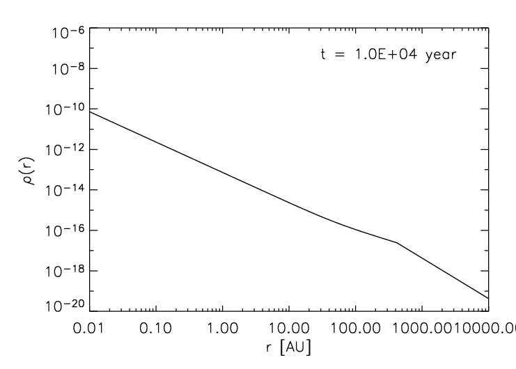
2. Plot the profiles \(\rho (t_0)\) for four different times with a double-logarithmic scale.

3. Plot the mass of the protostar M(t) against the time.

4. Write a program that determines the accretion rate of the forming protostar and plot it against time. Use, for example, the change in mass in the .sink file. Compare your results with those of Shu.

4.3 Simulations with rotation velocity field

1. Explain first what changes for the accretion in simulations with a rotation velocity field and why this is physically meaningful.

2. Create two-dimensional density plots of the areas of interst. You will notice that an accretion disk forms around one or more protostars. For the initial time also plot velocity vectors.

3. Identify the accretion disks.

4. Check whether these disks are Keplerian.

5. Plot \(\rho\)(r) and M(t).

6. Plot the accretion rate against the time.

7. Explain how and why the accretion rate changes compared to simulations without a velocity field.

8. Determines the ratios \(\alpha = \dfrac{E_{therm}}{E_{grav}}\) and \(\beta = \dfrac{E_{rot}}{E_{grav}}\). Explain how the simulation changes if one varies \(\alpha\) and \(\beta\) .

4.4 Simulations with turbulent velocity field

1. First, explain why even in simulations with turbulent velocity fields accretion disks usually occur.

2. Plot \(\rho\)(r) and M(t) and compare this with the other simulations.

3. Plot the accretion rate against the time and compare them with the accretion rates of the other simulations.

4. Create with "Splash" a two-dimensional density plot for different times. For the initial time, also plot velocity vectors. Describe what can be seen?

5. Optional: Create a video clip. In order to do this, create with Slash for each time step a "png" and put them together in a video.

5 Manual

In this section, the usage of the two programs Phantom and "Splash" is explained in detail. If you are running a Linux or Mac machine, these programs can easily be installed. In case of a windows machine it is reccomended to use the installation provided in the CIP pool.

5.1 Phantom

Phantom is an SPH code, running in modern FORTRAN. This short introduction should equip you with everything you need. In case something remains unclear or you want to get some additional information, please see the documentation.

To start the simulation, the initial conditions must be specified. For this experiment we will use the predefined r2sphere- and cluster-setup. The first one can be used for parts 5.1 - 5.3. The latter is only required for 5.4. In each case, the particles are placed as desired and only some parameters have to be specified. In the following this is explained in detail. In case you want to dive right in, 6 summarizes the following discussion.

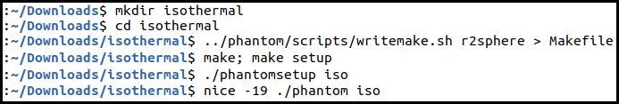
Using the r2sphere-setup as an example, create a folder and change to this folder. Type the follwing command in the terminal.

  ~/path/to/phantom/scripts/writemake.sh r2sphere > Makefile

This will create a makefile in your current directory. With

  make; make setup

the phantom initializer and the executable are loaded. Using phantomsetup the initial conditions can be set interactively via the terminal. Run it by typing

  ./phantomsetup myproject

Do not worry, in case of a typo you can chang the input in the myproject.setup file before continuing with the next step. Edit it and execute the command again. In addition the program writes a myproject.in file. This file defines parameters for the actual calculation. Most importantly for you, the runtime parameters can be manipulated here.

After successfully editing the myproject.in file, the actual computation is started by typing

  nice -19 ./phantom myproject.in

The nice -19 command lowers the priority of the code to ensure proper usability of the computer, while the code is executed. 6 summarises the commands needed.

The computation creates four different types of files. The first one, a .ev file (environment), contains global parameters like the energy of the system. It is in plain text format and can be read easily into any programming language. The same applies to the .sink file, which contains all information about the sink particles. The third type is the most important one, the dump files. They contain all information about the particles and can be evaluated either by Splash, which will be introduced in the next chapter or read into python via a script (/phantom/scripts/readPhantomDump.py). It contains several useful functions, but most importantly you want to use the read_dump function, which writes all information in the dump file into a dictionary. If you wish to use Julia, the phyton script can be included via the PyCall library. General information, such as time and units, can be found in the "quantities"-key, and the data for the particles themselves are stored in the "blocks" section. Once a sink particle is created there will be two blocks, One for the gas and one for the sink particles. There are two things to keep in mind. First of all, the density is not stored in the dump files to save storage. Therefore, it has to be calculated from the smoothing length. Secondly, accreted particles are marked with a negative smoothing length. Make sure to exclude them in your analysis.

5.2 Splash

The simulations can be analyzed graphically with the program "Splash". Open the terminal in the folder containing the simulation results. "Splash" is called via the command:

  ssplash myproject_0*

(in never version of Splash the command reads splash, not ssplash ). The ending "*" tells the program to load all timesteps, e.g. with "myproject_00001" just the first file is loaded.

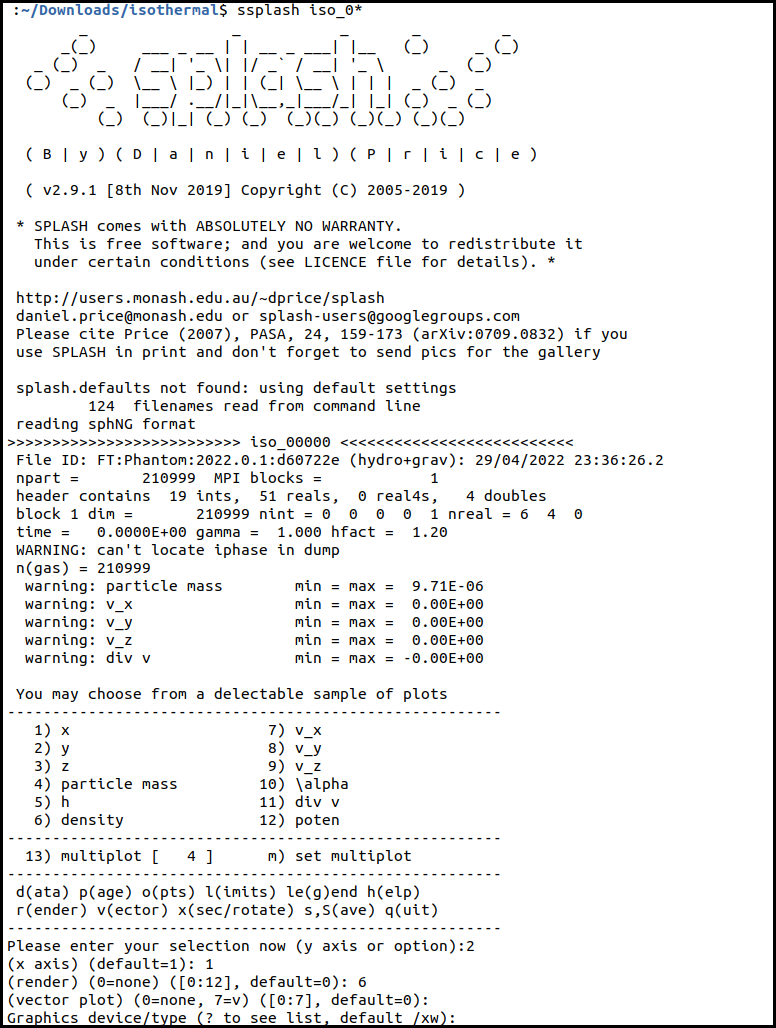
Splashs interactive menu offers a variety of settings. The following covers only the very basics. In order to create a one-dimensional plot, one simply has to assign the properties to the axis. For example, x = 1 and density = 6. For a two-dimensional render plot, one has to assign y to the Y-axis, x to the X-axis, and chose the third property, for example, the density(6) (figure7).

With the default settings, the plots are called within the interactive mode. Here you can move with "b" and "space" between the different time steps. With "l" you apply a logarithmic scale to the axis. The settings are saved with "s". One leaves the interactive mode with "q".

The plots are saved if you type "/png" instead of the default "Graphics device/type" "/xw" (interactive mode). Several plots can be morphed into a movie by the following command:

  ffmpeg -i splash_%04d.png movie.mp4

Splash is, just like Phantom, a very complex program, which offers a huge set of tools. If you want to create nice plots using Splash, it is recommended to use the documentation (there are many useful hints, like this one).

References

Materials

• Instruction PDF
• Git-repository for the Phantom library