
Agent-based modeling
1 Theory
1.1 Transport and traffic
Transport problems appear in a large variety of physical systems. Electrical current, which means transport of electrons from an cathode to an anode, is an indispensable part of our daily lives that we are well aware of. Another process that we crucially rely on – maybe less consciously – is intracellular transport that is carried out by molecular motors. Molecular motors are proteins that move along filaments in our cells by converting chemical into mechanical energy. And transport is not restricted to the microscopic world: Car traffic is an example of transport in the macroscopic world, which exhibits interesting phenomena that we are going to address within this lab course project.
The transport problems sketched above constitute a class of genuine non-equilibrium systems. The existence of transport, i.e., currents, immediately implies that the principle of detailed balance – a defining feature of equilibrium states – is broken. This means that by studying transport problems we venture into a regime where the established rules and concepts of equilibrium statistical physics are not necessarily applicable any more. In this regard, you will find within this project that on the one hand some concepts can be generalized to non-equilibrium settings, while on the other hand rules that hold in equilibrium can be broken out of equilibrium.
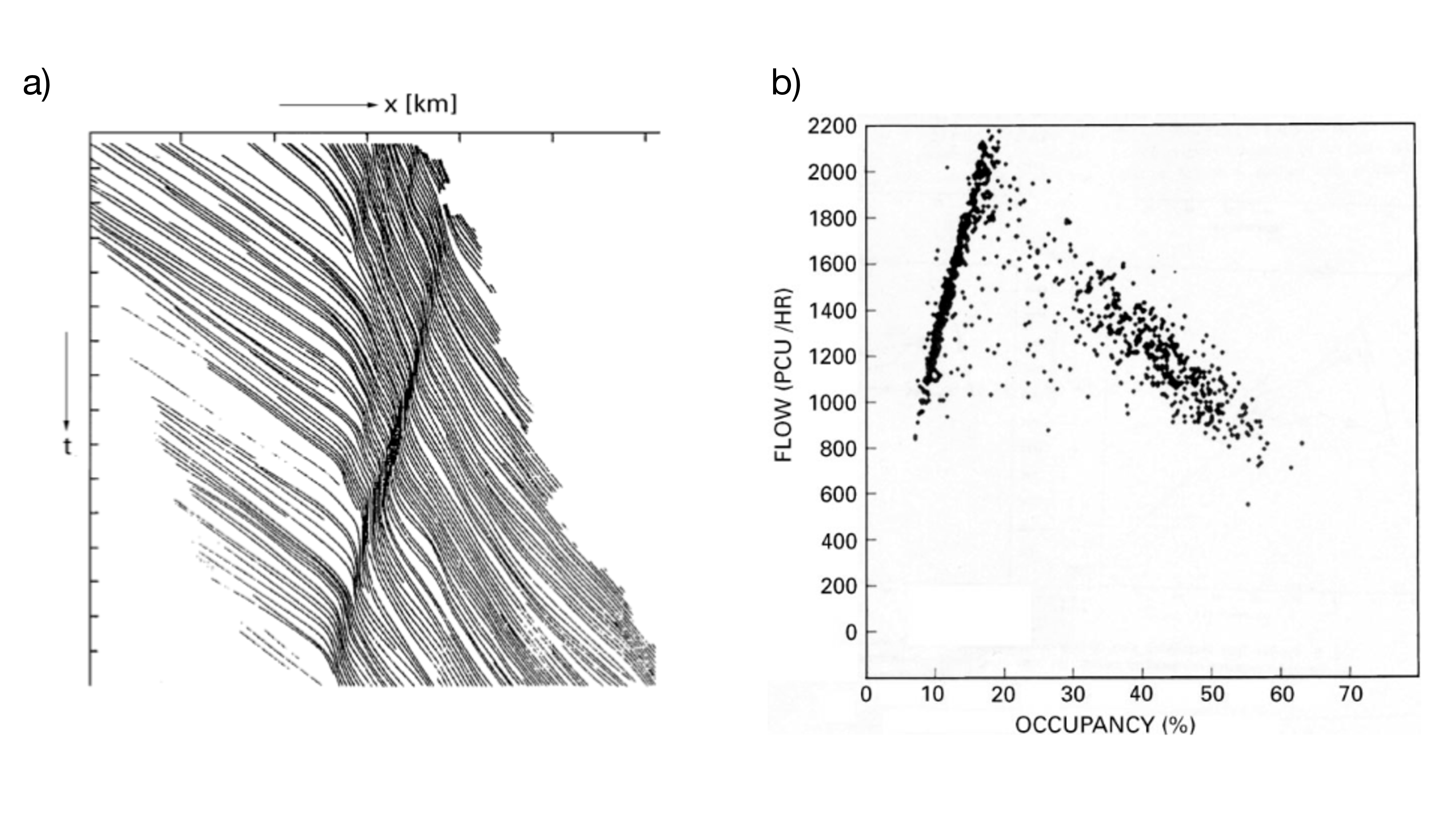
A phenomenon occurring in car traffic, which is particularly intriguing to the scientist and annoying to the traffic participant, is the spontaneous formation of jams without any apparent reason. An example of this is shown in Fig. 1, which displays the trajectories of individual vehicles on one lane of a multi-lane highway. Initially, the traffic flows freely, but then a dense region appears due to fluctuations. This dense region becomes a jam, where vehicles even have to stop, before it eventually resolves again. The diagram clearly reveals a backward propagation of the jam against the driving direction. It is today established that this backward propagation of car traffic jams has a characteristic velocity of about 15km/h, which can be used to calibrate theoretical models [3].
Fig. 1 revealed already that the formation of jams is related to the density of vehicles on the road. A central tool to analyze this relation is the so-called fundamental diagram in which the traffic flow (or the current) is plotted against the density of vehicles. An example from empirical traffic data is shown in Fig. 1. It clearly shows the attenuation of the flow with increasing density, which we can relate to the formation of congustion. Reversely, there is a linear relation between flow and density at small occupancies, where the traffic flows freely. The reason for this is that any additional vehicle contributes to the flow when the road is free. More formally, the average velocity does not vary with density at low densities and, thereby, the hydrodynamic relation \[J=\rho v \qquad{(1)}\] yields the linear relation between current and density.
Closer inspection of Fig. [fig:empirical_fd] shows that there are, in fact, also characteristic differences in the fluctuations of the data points depending on the density, which arise, because the data corresponds to observations of restricted space-time windows. In the free flow regime the fluctuations around the increasing line are very small, whereas the data points spread out much more irregularly over a large area at larger occupancies.
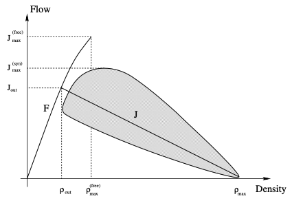
The above observations lead to the distinction of three different phases of traffic flow shown in the schematic fundamental diagram in Fig. 2: In free flow interactions between vehicles are rare. Cars move with their desired velocity and flow increases linearly with density. More detailed analysis reveals that states with flows larger than \(J_{\text{out}}\) form a metastable branch. All states not of free flow type are called congested states. They are characterized by an average velocity smaller than the desired velocity of the drivers. Two congested phases can be distinguished. Wide jams are regions of high density and negligible average velocity and flow. In synchronized flow the average velocity is significantly lower than in free flow, but the flow can be much larger than in wide jams. Characteristic for the congusted phases is the absence of a functional flow-density relation and data points are spread irregularly over a 2d area.
The objective of this project is to investigate minimal models that describe car traffic in order to understand the mechanisms that cause these characteristic features.
1.2 Asymmetric Simple Exclusion Process (ASEP)
Generally, the transport phenomena discussed in Section 1.1 can be modeled in the framework of driven diffusive systems, where the drive produces the directed currents and diffusion refers to stochastic contributions due to a coupling to an environment or uncontrolled behavior of the drivers.
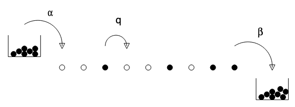
The Asymmetric Simple Exclusion Process (ASEP) is the “drosophila” model of driven diffusive systems. It describes the discretized motion of particles in one dimension, where each spatial position cannot be occupied by more than a single particle (the exclusion principle). Each discrete time step corresponds to applying a simple update rule: Each particle moves to its empty right neighbor site with probability \(q\). Reversely, particles stay at their site if the right neighbor site is occupied or with probability \(1-q\). In addition, when considering open boundary conditions, a particle is filled into the empty first site with probability \(\alpha\) and removed from the occupied last site with probability \(\beta\). Physically, this corresponds to a coupling to reservoirs at both ends that act as source or sink, respectively, for the particles. The whole process is shown pictorially in Fig. 3. We will be interested in the characteristic features of the steady state of this process that is reached a sufficiently long time after its initialization.
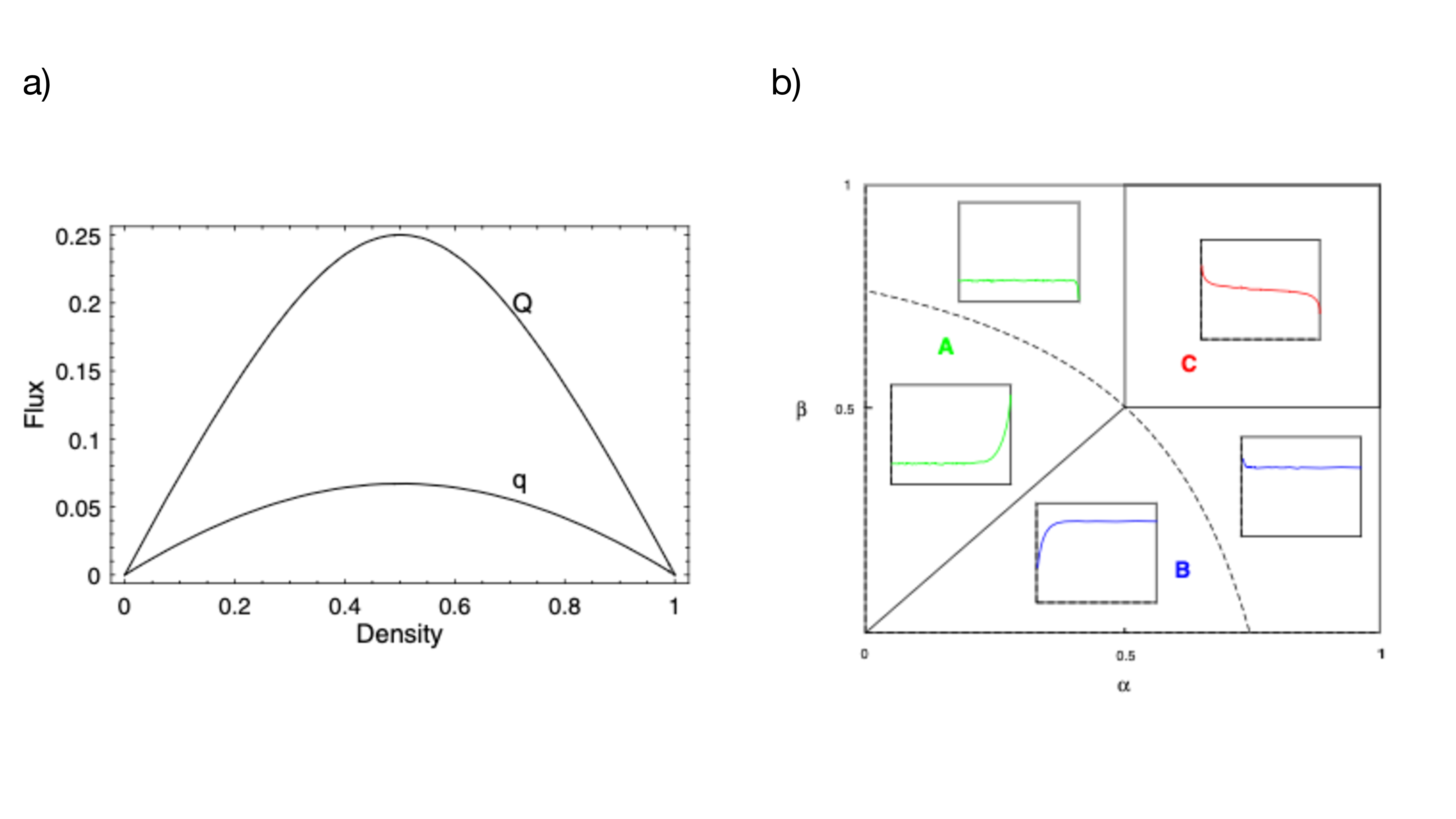
We denote the occupation of site \(l\) in the one-dimensional lattice at time step \(t\) by \(x_l^t\). Assuming periodic boundary conditions the local density at site \(l\), \(\rho_l\), has to become uniform and equal to the global density \(\rho\) in the steady state, i.e., \[\lim_{t\to\infty}\rho_l(t)=\lim_{t\to\infty}\langle{x_l^t}\rangle=\rho\ .\qquad{(2)}\] If we assume in addition that the occupation of each lattice site is independent of the occupation of the neighboring lattice sites, the hydrodynamic relation 1 in the steady state can be written as \[J(\rho)=\rho v(\rho)=q\rho(1-\rho)\ .\qquad{(3)}\] Here, we used that the velocity of a particle at site \(l\) is given by its probability to move in the current time step. This probability, in turn, is the probability of finding the next site empty and moving. Therefore, \(\langle{v_l}\rangle=q(1-\langle{x_{l+1}}\rangle)=q(1-\rho)\) under the aforementioned mean-field assumptions. Fig. 4 shows the corresponding fundamental diagram for two different values of \(q\).
The phenomenology of the ASEP becomes richer, when considering open boundary conditions. In fact, different phases are realized depending on the values of \(\alpha\) and \(\beta\). The corresponding phase diagram is shown in Fig. 4b). It exhibits a low density phase (A), a high density phase (B), and a maximal current phase (C). The low density phase is characterized by a density \(\rho<1/2\) far away from the boundaries (bulk-density) and a current that depends only on \(\alpha\). In the high density phase, \(\rho>1/2\) in the bulk and the flow depends only on \(\beta\). In the maximal current phase, the density at site \(L/2\) equals \(1/2\) and the current depends only on \(q\). Fig. 4b) moreover includes exemplary density profiles, i.e. plotting the density for each site \(\rho_l = \langle x_l \rangle\), for the different regions of the phase diagram in the steady state. These profiles reveal that the phases A and B can be further separated according to the excess density at either end of the system.
1.2.1 Update schemes
The above definition of the discrete ASEP does not specify how to perform the update steps in detail. In fact, there are four possible choices:
Parallel update: Apply the update rule in parallel to all particles given the current configuration.
Sequential update: Apply the update rule each individual particle sequentially in a fixed order.
Shuffle update: Apply the update rule each individual particle sequentially in a random order that changes from time step to time step. This procedure corresponds to drawing without putting back in the urn model language.
Random sequential update: Apply the update rule to a randomly chosen particle. Repeat this \(N\) times, where \(N\) is the total particle number in the system. This procedure corresponds to drawing with putting back in the urn model language, meaning that one particle can also be moved multiple times or not at all within one time step.
It turns out that the choice of the update scheme can affect its physical properties. Exploring the behavior of different update schemes will be part of this lab course project.
1.3 Nagel-Schreckenberg model (NaSch)
While the ASEP is appealing for its simplicity and the existence of analytical solutions, it clearly lacks features of real world traffic. For example, on a real road cars travel with different non-zero velocities and drivers do not always adhere to an optimal and deterministic policy for acceleration and deceleration. The Nagel-Schreckenberg (NaSch) model can be viewed as a generalization of the ASEP that includes such features. We again consider a discretized one-dimensional road occupied by \(N\) cars and with periodic boundary conditions. Each car is characterized by its velocity \(v_n=0,1,\ldots,v_{\text{max}}\). Moreover, denoting the position of the \(n\)-th car by \(x_n\), we define its headway as \(d_n=x_{n+1}-x_n-1\) (cars are labelled according to their order on the road). Then, the update rule for each discrete time step of the NaSch model, which is applied in parallel to all cars, is
Acceleration: If \(v_n<v_{\text{max}}\), velocity is increased by \(1\), i.e., \(v_n^{(1)}=\text{min}(v_n+1,v_{\text{max}})\).
Deceleration (to avoid crashes): If \(d_n<v_n^{(1)}\), velocity is reduced to \(d_n\), i.e., \(v_n^{(2)}=\text{min}(v_n^{(1)},d_n)\).
Randomization: If \(v_n^{(2)}>0\), velocity is decreased randomly by \(1\) with probability \(p\), i.e., \[v_n^{(3)}= \begin{cases} \text{max}(v_n^{(2)}-1,0)&\text{with probability }p,\\ v_n^{(2)}&\text{with probability }1-p. \end{cases}\qquad{(4)}\]
Vehicle movement: Each car is moved forward according to its new velocity \(v_n=v_n^{(3)}\) determined in steps 1-3, i.e., \(x_n\to x_n+v_n\).
Step 1 expresses the desire of the drivers to move as fast as possible (or allowed). Step 2 reflects the interactions between vehicles and guarantees the absence of collisions in the model. Step 3 incorporates many effects, e.g. natu- ral fluctuations in the driving behaviour. It is responsible for spontaneous jam formation since it can lead to the chain reactions described above. Finally, in Step 4 all cars will move with their new velocity as determined in the first three steps. This set of rules is minimal in the sense that every subset or change in the order will no longer produce realistic behaviour, e.g. spontaneous jams.
The NaSch model includes a random deceleration to account for stochastic imperfections in the drivers actions in the form of unnecessary braking. The model can be slightly extended to the so-called Velocity-Dependent-Randomization (VDR) model by making the randomization parameter velocity-dependent, \(p\equiv p(v)\). Then, the probability for random deceleration is computed in an initial step according to
Determination of the randomization parameter: The randomization parameter for the \(n\)-th car is given by \(p_n=p(v_n(t))\).
With this, a slow-to-start rule can be implemented through \[p(v)=\begin{cases}p_0&\text{for }v=0,\\p&\text{for }v>0,\end{cases}\qquad{(5)}\] with \(p_0>p\). This means that cars that have been standing in the previous time step are more likely to brake than cars that are moving - or, looked at another way, have a delay in accelerating once the lane clears.
2 Preparation
2.1 Theory
While you familiarize yourself with the theoretical background, find answers to the following questions:
It was claimed in the introduction that some concepts of equilibrium statistical physics can be generalized to non-equilibrium situations, while some equilibrium rules can be broken away from equilibrium. Can you give an example for each case based on the model systems that you will address?
What could be suited order parameters to distinguish the different phases shown in Fig. 4b)? Can you devise suited scalar quantities that you could use to distinguish the different types of density profiles within phases A and B?
How can you estimate the probability \(p\) in the NaSch model by observing the behavior of spontaneous jams?
2.2 Coding
In this lab course project you will write your own implementation of the traffic simulations. When composing your simulation, consider the following hints:
A central observable in this project is the current \(J\), which can be computed from a given mean velocity \(v\) and density \(\rho\) via the hydrodynamic relation 1. How can you extract \(\rho\) and \(v\) for this purpose from the representation of the state of the system that you will use in your code?
It is in principle possible to formulate all models discussed in Section [sec:theory] in a unified framework. How can you translate the ASEP model into the language of the NaSch model?
How can you test the correctness of your code?
3 Tasks
3.1 ASEP with periodic boundary conditions
Run the simulation for a suited grid of values for \(q\) and \(\rho\) using the four different update rules.
Plot a few exemplary space-time diagrams for all update schemes, including the case \(q=1\), \(\rho=0.5\). Describe them qualitatively and discuss differences between the update schemes. Can you identify the spontaneous formation of jams?
For all update schemes, plot the fundamental diagram for the different values of \(q\) using averages over large spatio-temporal regions in the steady state (check for convergence). How do your numerically obtained diagrams compare to the mean-field prediction?
3.2 ASEP with open boundary conditions
Choose three suited values of \(\alpha\) and \(\beta\), respectively, and inspect the local density profile \(\rho_i\) in the stationary state. How many iterations are required to obtain converged profiles?
Plot the exemplary steady state density profiles and discuss the qualitative differences. Include data that demonstrates convergence.
Plot the density and current in the stationary state for the grid of values for \(\alpha\) and \(\beta\). Can you identify the phase boundaries as in Fig. 4b)?
Perform simulations for the steady state density profiles on a suited grid of values for \(\alpha\) and \(\beta\). Use shorter simulations and a smaller system size to first fix a suited value for \(q\) and the grid resolution.
Extract the quantities you devised in [q2] to characterize the shape of density profiles. Plot the values in the \(\alpha\)-\(\beta\)-plane. Can you identify transitions lines? How do they compare to Fig. 4b)?
3.3 NaSch
Compute space-time trajectories for a suited grid of \(\rho\) and \(p\).
Plot a few exemplary space-time diagrams. Describe them qualitatively and discuss how they compare to the space-time diagrams of the ASEP. Can you identify the spontaneous formation of jams?
Assuming that all vehicles in your simulation are cars, estimate a realistic value for \(p\) based on the space-time diagrams.
Plot the fundamental diagram for the different values of \(p\) using averages over large spatio-temporal regions in the steady state (check for convergence). Can you identify the different phases of traffic flow?
3.4 VDR
Compute space-time trajectories for a suited grid of \(\rho\) and \(p\) with a fixed \(p_0\) of your choice.
Plot a few exemplary space-time diagrams for \(p_0 \gg p\). Describe them qualitatively and discuss how they compare to the space-time diagrams of the NaSch model.
Plot the fundamental diagram for different initial-conditions. What is the influence of the simulation-time and can you identify the metastable states observerd in real traffic?
3.5 (Optional) Further model extensions
What are further extensions of the traffic model that could be interesting? Choose one that you implement and discuss how the new ingredients change the properties of the resulting traffic flow.