
Molecular dynamics
1 Theory
1.1 Introduction
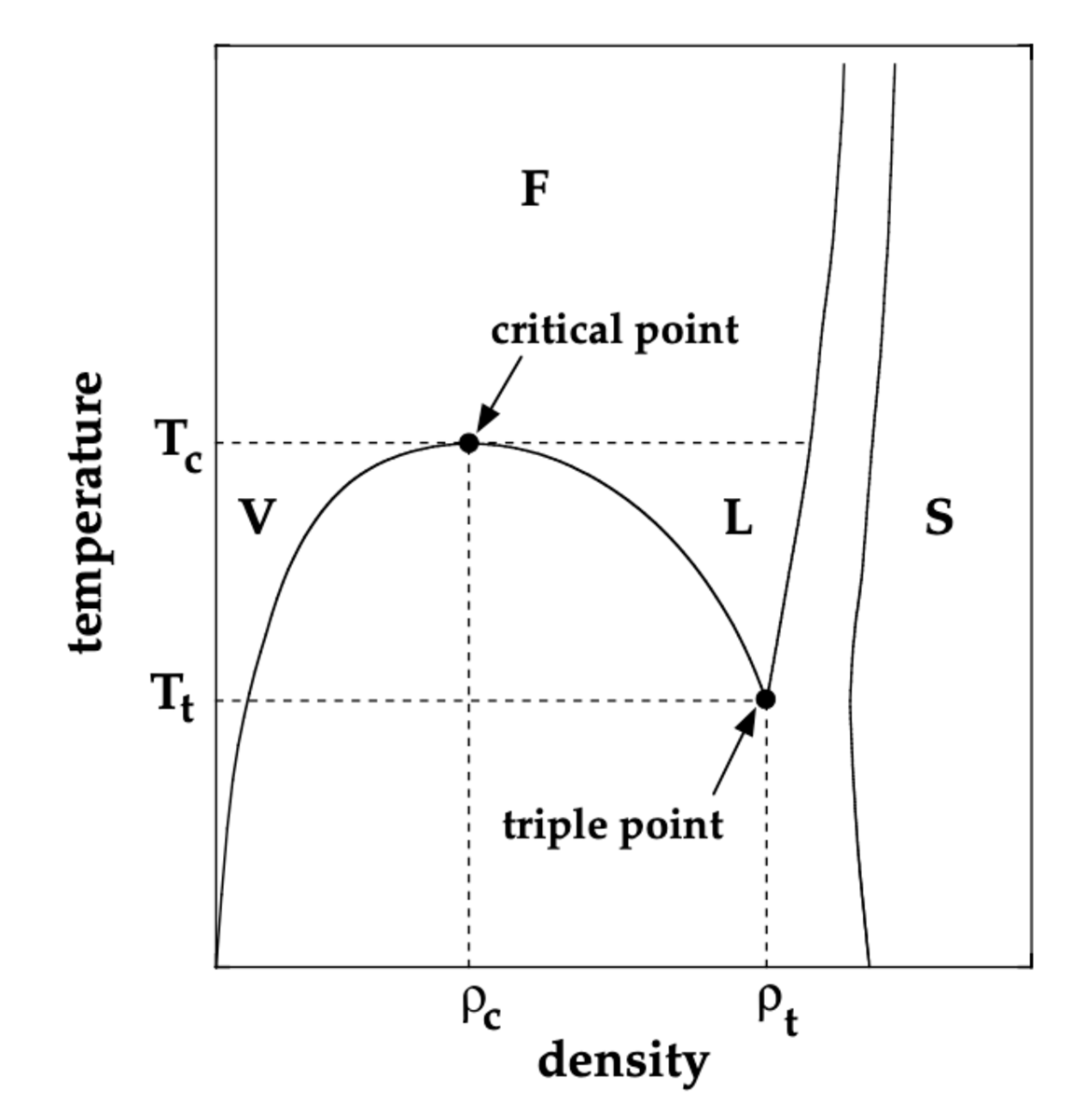
When studying the thermodynamic properties of many microscopic particles that can move freely in space, the simplistic model of the ideal gas yields many insights allowing us to understand the gaseous state of matter. However, this model clearly reaches its limitations once interactions between the particles become relevant at high enough densities \(\rho\) and low enough temperatures \(T\). In the presence of interactions the characteristics of the system can change and it can transition into a liquid or solid state of matter. A schematic phase diagram in the \(\rho-T\)-plane is shown in Fig. 1. At temperatures below the critical temperature \(T_c\) it indicates a gaseous phase (V) at low densities and a liquid phase (L) at intermediate densities. In between lies a coexistence region, where both states are stable and at temperatures \(T>T_c\) both transition into a fluid state, through which gas and liquid can be continuously connected. The solid state (S), in which particles arrange on a regular lattice, is reached at high densities.
For the microscopic description of these states of matter we can assume a classical Hamilton function for \(N\) identical particles with mass \(m\) of the form \[ \mathcal H(\mathbf p, \mathbf r)=\mathcal K(\mathbf p)+\mathcal V(\mathbf r)=\sum_{i=1}^N\frac{p_i^2}{2m}+\sum_i\sum_{j>i} V_2(|\mathbf r_i-\mathbf r_j|)\ .\qquad{(1)}\] Here, \(\mathbf r,\mathbf p\in\mathbb R^{3N}\) denote the positions and momenta of the particles, respectively. \(\mathcal K\) is the kinetic energy and \(\mathcal V\) denotes the potential energy contributions due to the interactions between the particles. In the second equality, we introduce the pair potential \(V_2(r)\) indicating that the relevant interactions are pair-wise interactions that only depend on the distance between the particles. With \(\mathbf r_i\in\mathbb R^3\) we denote the coordinate vector of particle \(i\).
The separation of the Hamilton function into the momentum-dependent kinetic part and the position-dependent potential part implies that the partition sum of the system factorizes accordingly. This means, that all thermodynamic properties of the system can be cast as a sum of these two contributions. In particular, the three different states of matter can be characterized by the relation of the magnitudes of the two energy contributions. In the dilute gas, \(\langle\mathcal K\rangle\gg\langle\mathcal V\rangle\), while in the solid state the potential part dominates, \(\langle\mathcal K\rangle\ll\langle\mathcal V\rangle\). The liquid state is characterized by comparable magnitude of both contributions, \(\langle\mathcal K\rangle\approx\langle\mathcal V\rangle\).
Here, the brackets \(\langle\cdot\rangle\) denote the thermodynamic expectation value in the equilibrium state, i.e., for some observable \(O(\mathbf p,\mathbf r)\), \[\begin{aligned} \langle O(\mathbf p,\mathbf r)\rangle=\frac{1}{Z}\sum_{\mathbf p,\mathbf r}\mathcal P(\mathbf p,\mathbf r) O(\mathbf p,\mathbf r)\ , \end{aligned}\qquad{(2)}\] where \(\mathcal P(\mathbf p,\mathbf r)\) denotes the probability of the microscopic state in the thermodynamic ensemble, and \(Z=\sum_{\mathbf p,\mathbf r}\mathcal P(\mathbf p,\mathbf q)\) is the partition sum. In order to compute such expectation values numerically, we will rely in this project on the ergodic property of interacting many-body systems, which means that the equilibrium expectation values are equal to long time averages when following the dynamics of the system, \[\begin{aligned} \langle O(\mathbf p,\mathbf r)\rangle=\lim_{\tau\to\infty}\frac{1}{\tau}\int_{t_0}^{t_0+\tau}dt\ O(\mathbf p(t),\mathbf r(t))\ . \end{aligned}\qquad{(3)}\] The underlying trajectories \((\mathbf p(t),\mathbf r(t))\) follow the Hamiltonian equations derived from Eq. 1, \[\begin{aligned} \dot r_k = \frac{\partial\mathcal H}{\partial p_k}=\frac{p_k}{m}\ ,\quad\dot p_k = -\frac{\partial\mathcal H}{\partial r_k}\ , \end{aligned}\qquad{(4)}\] or, equivalently, Netwon’s equation of motion \[\begin{aligned} m\ddot r_k &= F_k(\mathbf r) = -\frac{\partial}{\partial r_k}\mathcal V(\mathbf r)\ . \end{aligned}\qquad{(5)}\]
1.2 Lennard-Jones potential
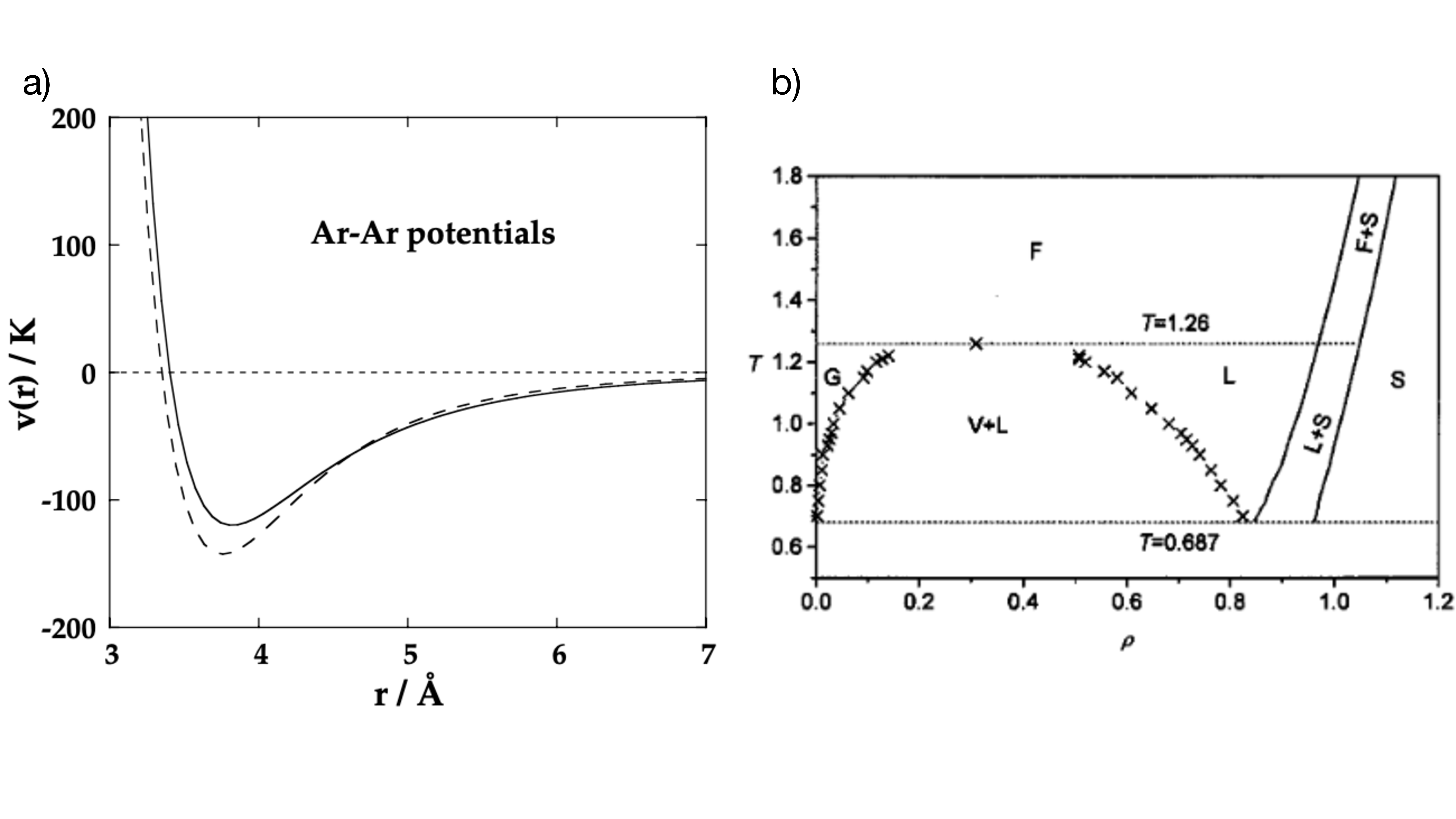
In this project we will focus on a system composed of atoms (not molecules). In particular, we will consider Argon atoms, for which the pair potential is shown with a dashed line in Fig. 2a). The key features of the potential are a strong repulsion at short distances, an attractive minimum at intermediate distance, and a decay towards zero at large distance. The repulsion at short distances originates in overlapping electron orbitals. The attractive component corresponds to a van-der-Waals force that arises due to the interaction of mutually induced dipoles; as such it decays with the sixth power of distance.
The solid line shows the so-called Lennard-Jones potential \[\begin{aligned} V_{LJ}(r)=4\epsilon\bigg[\Big(\frac{\sigma}{r}\Big)^{12}-\Big(\frac{\sigma}{r}\Big)^6\bigg] \end{aligned}\qquad{(6)}\] and we can see that the suitably chosen parameters \(\epsilon\) and \(\sigma\) give a good agreement with the actual potential. This is the functional form of the potential that you will consider for the purpose of this project. In simulations the potential is typically cut off at a suitably chosen cutoff-distance \(r_c\), i.e., \[\begin{aligned} V_{LJ}(r)= \begin{cases} 4\epsilon\bigg[\Big(\frac{\sigma}{r}\Big)^{12}-\Big(\frac{\sigma}{r}\Big)^6\bigg]&\text{if }r\leq r_c\\ 0&\text{if }r>r_c \end{cases} \ . \end{aligned}\qquad{(7)}\]
The phase diagram of the Lennard-Jones model in the \(\rho-T\) plane has been investigated by numerical simulations and an exemplary result is shown in Fig. 2b). The diagram exhibits the same features as the schematic diagram in Fig. 1. All quantitative values are given in the natural Lennard-Jones units, which will be discussed in the following subsection.
1.2.1 Reduced units
The Lennard-Jones potential 6 provides us with a natural choice for the unit of length and the unit of energy to use in our computer simulation, namely \(\sigma\) and \(\epsilon\). This means, that the simulations are performed with dimensionless parameters \(\epsilon_{LJ}=1\) and \(\sigma_{LJ}=1\). Here, we added the subscript \(LJ\) to indicate that these quantities are given in dimensionless Lennard-Jones units or reduced units. When a simulation is performed in these units, the result is applicable to any physical system that can be modeled using the Lennard-Jones potential by translating the units.
For example, the dimension of pressure is [energy/volme], and, therefore the pressure of Argon would be obtained from the simulation in Lennard-Jones units as \[\begin{aligned} \frac{P_{Ar}}{\epsilon_{Ar}/\sigma_{Ar}^3} = P_{LJ} \end{aligned}\qquad{(8)}\]
Similarly, \(k_BT_{LJ,c}\) is an energy and the Boltzmann constant \(k_B\) can independently be chosen dimensionless to be \(k_{B,LR}=1\). From this, the critical temperature of Argon is obtained by rescaling with the Argon unit of energy \(\epsilon_{Ar}\), \[\begin{aligned} \frac{k_B T_{Ar,c}}{\epsilon_{Ar}}=T_{LJ,c} \end{aligned}\qquad{(9)}\]
By inspecting Eq. 1 we find \(m\) as another independent simulation parameter, which has dimension [mass]. The choice \(m_{LJ}=1\) defines the Lennard-Jones unit of mass. Now that we defined the units of energy, length, and mass, we can derive the Lennard-Jones unit of time \[\begin{aligned} \tau_{LJ} = \sqrt{\frac{m_{LJ}\sigma_{LJ}^2}{\epsilon_{LJ}}}\ , \end{aligned}\qquad{(10)}\] for example, because we know that the dimension of kinetic energy corresponds to [mass\(\times\)length\(^2\)/time].
1.3 Observables of interest
In this section we summarize various quantities of interest for the characterization of the Lennard-Jones fluid. Further details and derivations can be found, e.g., in [1]. All relations are given in dimensionless units, especially the Boltzmann constant \(k_B=1\) and mass \(m=1\).
1.3.1 Thermodynamic and statistical properties
A central quantity of interest is the temperature \(T\). In equilibrium the temperature is related to the kinetic energy via the equipartition theorem for point-like particles as \[\begin{aligned} T=\frac{2}{3(N-1)}\langle \mathcal K\rangle\ . \end{aligned}\qquad{(11)}\]
To compute the pressure from given phase space coordinates, we can resort to Clausius’ virial theorem. The virial is defined as \(W=\langle\sum_k r_k\dot p_k\rangle\), i.e., the sum of each spatial coordinate multiplied by the force acting on the corresponding degree of freedom. According to the virial theorem, \(W=-3NT\). Hence, for an ideal gas with equation of state \(PV=NT\), we immediately obtain \(W=-3PV\), and the forces are solely due to the interaction with the container.
In an interacting system we have to add to the ideal gas part the forces induced by the interaction potential \(\mathcal V(\mathbf r)\), yielding \[\begin{aligned} W&=-3PV+\big\langle\sum_k r_k\ \frac{\partial\mathcal V(\mathbf r)}{\partial r_k}\big\rangle=-3NT \nonumber\\ \Leftrightarrow P&=\frac{1}{V}\Big(NT-\frac{1}{3}\big\langle\sum_k r_kF_k\big\rangle\Big)\ . \end{aligned}\qquad{(12)}\]
Finally, in equilibrium, the distribution of individual particle velocities follows the Maxwell-Boltzmann distribution \[\begin{aligned} P_T(v)=4\pi\bigg(\frac{1}{2\pi T}\bigg)^{\frac{3}{2}} v^2e^{-\frac{v^2}{2T}}\ . \end{aligned}\qquad{(13)}\]
1.3.2 Correlations in space and time
An important correlation function that characterizes the spatial distribution of particles is the two-particle distribution function \(g^{(2)}(r)\) that indicates the probability of finding another particle at distance \(r\) from a fixed one. \(g^{(2)}(r)\) is normalized to the volume element, i.e., it is related to the plain distribution function \(n(r)\) via \[\begin{aligned} n(r)\ dr=4\pi r^2\rho g^{(2)}(r)\ dr \end{aligned}\qquad{(14)}\]
An interesting correlation function that characterizes spatio-temporal fluctuations is the squared distance travelled by a fixed particle in a given time, \[\begin{aligned} \Delta^2(t)=\big\langle |\mathbf r_i(t)-\mathbf r_i(0)|^2\big\rangle\ . \end{aligned}\qquad{(15)}\] Due to the interactions, the motion of the particles is expected to be diffusive on long time scales, meaning that \(\Delta^2(t)\) grows linearly at large \(t\) with a slope given by the self-diffusion coefficient \[\begin{aligned} D=\lim_{t\to\infty}\frac{1}{6t}\Delta^2(t)\ . \end{aligned}\qquad{(16)}\] On the other hand, \(\Delta^2(t)\) can be reformulated as a velocity correlation function. By inserting \(\mathbf r_i(t)-\mathbf r_i(0)=\int_0^t\mathbf v_i(t')\ dt'\) in Eq. 15 one can derive that \[\begin{aligned} D=\int_0^\infty Z(t)\ dt \end{aligned}\qquad{(17)}\] with the velocity autocorrelation \[\begin{aligned} Z(t) = \frac{1}{3}\langle \mathbf v_i(t)\cdot\mathbf v_i(0)\rangle\ . \end{aligned}\qquad{(18)}\] Notice that according to the equipartition theorem \(Z(0)=T\).
Since the two-particle distribution function allows us to compute observables that depend only on the distance of particles, we can derive a relation between \(g^{(2)}(r)\) and the velocity autocorrelation. Short-time expansion of Eq. 18 leads to \[\begin{aligned} Z(t)=T\big(1-\Omega_0^2\frac{t^2}{2}+\ldots\big) \end{aligned}\qquad{(19)}\] with \[\begin{aligned} \Omega_0^2=\frac{1}{3T}\langle \dot{\mathbf v}_i\cdot\dot{\mathbf v}_i\rangle=\frac{1}{3T}\langle |\mathbf F_i|^2\rangle =\frac{4\pi\rho}{3T}\int_0^\infty |\nabla_{\mathbf r_i} V_2(r)|^2 g^{(2)}(r) r^2\ dr\ . \end{aligned}\qquad{(20)}\]
1.4 Molecular dynamics simulations
1.4.1 Velocity Verlet algorithm
The core of a molecular dynamics simulation is the numerical integration of the equations of motion 4. A suited algorithm for this purpose is the velocity Verlet algorithm that gives the following prescription to update the phase space coordinates with a time step \(\Delta t\): \[\begin{aligned} r_k(t+\Delta t) &= r_k(t)+\Delta t\ p_k(t) + \frac{\Delta t^2}{2}F_k(\mathbf r(t))\nonumber\\ p_k(t+\Delta t) &= p_k(t) + \frac{\Delta t}{2}\big[F_k(\mathbf r(t)) + F_k(\mathbf r(t+\Delta t))\big] \end{aligned}\qquad{(21)}\] This means that one first computes the update of the positions according to the first line. After that, one computes the forces \(F_k(\mathbf r(t+\Delta t))\) with the updated positions in order to then obtain the update for the momenta.
The local integration error of this scheme is \(\mathcal O(\Delta t^4)\). A sufficiently small time step \(\Delta t\) has to be chosen for accurate simulations. A good figure of merit for this purpose is energy conservation. In the absence of integration errors, the energy is an integral of motion of Hamiltonian dynamics. Deviations from energy conservation in the numerical simulation indicate too large time steps. For the Lennard-Jones problem a suited time steps lie around \(\Delta t\approx0.01\tau_{LJ}\).
1.4.2 Estimating ensemble averages
Due to the ergodicity of interacting many-body systems, the trajectories \((\mathbf p(t), \mathbf r(t))\) computed in a molecular dynamics simulation enable us to estimate thermodynamic ensemble averages (Eq. 2) through long time averages (Eq. 3).
We will now denote by \((\mathbf p^{(n)},\mathbf r^{(n)})\equiv(\mathbf p(n\Delta t), \mathbf r(n\Delta t))\) the phase space coordinates at the \(n\)-th of \(N_T\) discrete time steps. Then, we select from the whole sequence a sample \(\mathcal S=\{(\mathbf p^{(n)},\mathbf r^{(n)})|n>N_T-M\}\) with the sample size \(M\) chosen such that the initial transient dynamics of the system is excluded and we only consider the system in the equilibrated state. Then, we can estimate the thermodynamic expectation value of any observable \(O(\mathbf p, \mathbf r)\) as \[\begin{aligned} \langle O(\mathbf p, \mathbf r)\rangle = \overline O \equiv \frac{1}{M}\sum_{(\mathbf p, \mathbf r)\in\mathcal S}O(\mathbf p, \mathbf r)\ . \end{aligned}\qquad{(22)}\] Similarly, variances can be estimated as \[\begin{aligned} \sigma_O^2=\big\langle \big(O(\mathbf p, \mathbf r) - \langle O(\mathbf p, \mathbf r)\rangle\big)^2\big\rangle = \overline {O^2} - \overline O^2\ . \end{aligned}\qquad{(23)}\]
If \(O(\mathbf p^{(n)}, \mathbf r^{(n)})\) were uncorrelated random variables, the central limit theorem would tell us that the deviation of the estimate from the true mean is less than \(\Delta_O^M=\sigma_O/\sqrt{M}\). However, in our sample subsequent phase space points are clearly correlated, because they correspond to a continuous dynamics. The characteristic number of steps required for the decay of the autocorrelation is called the autocorrelation time \(\tau\).
If the autocorrelation time of the data is known, it can be used to define an effective number of uncorrelated samples, \(M_{\text{eff}}=M/(1+2\tau)\) [3]. With this, the error estimate becomes \[\begin{aligned} \Delta_O^M=\frac{\sigma_O}{\sqrt{M_{\text{eff}}}}=\frac{\sigma_O}{\sqrt{M}}\sqrt{1+2\tau_{ac}}\ . \end{aligned}\qquad{(24)}\]
For this purpose, it is required to estimate the autocorrelation time. A viable approach for this purpose is the binning analysis that is explained as part of the general purpose toolbox on the lab course website [4].
1.4.3 Boundary conditions
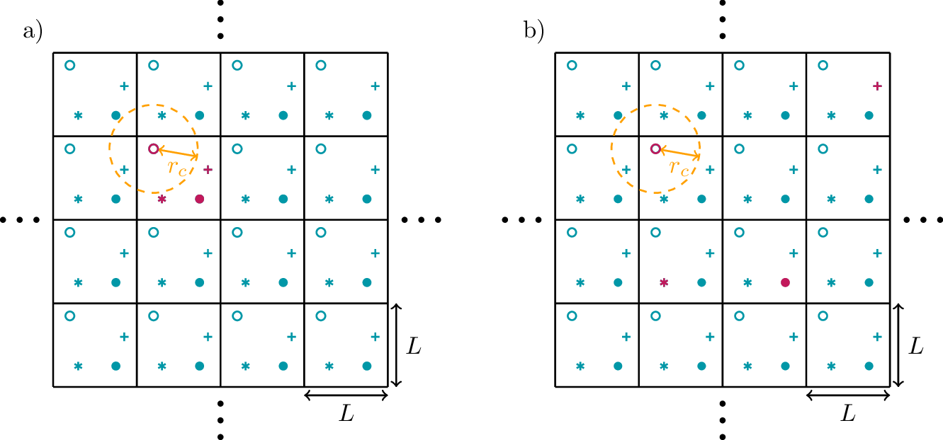
To avoid dealing with particles that collide with the walls of the container, it is useful to implement the simulation with periodic boundary conditions. This means that we define a simulation cube with linear extend L and volume \(V=L^3\), and we assume that beyond the boundaries of this cube the system configuration is repeated periodically. This situation is shown schematically in Fig. 3 for a two-dimensional case. Of all the particles shown only a small number corresponds to real particles in the simulation, namely those drawn in red. The other symbols correspond to fictitious copies of the simulated particles due to the periodic boundary condition. One typically initializes the particles such that they all reside in the same simulation cube as shown in Fig. 3a). However, during the time evolution the particles can cross the simulation cube boundaries, such that the simulated particles are scattered across different cubes as shown in Fig. 3b).
The orange circle surrounding the red circular particle o indicates the cutoff range of the interaction potential. This means, that the forces acting on o depend only on the positions of particles included in this radius. The finite size of the simulation cube becomes relevant when one particle is affected by the presence of multiple copies of another particle. Therefore, the simulation cube size has to be chosen substantially larger than the interaction range, \(L\gg r_c\).
To compute the forces acting on one particle, one has to identify all periodically translated fictitious copies of the other particles that lie within the interaction range. In the shown example for o, this corresponds to the fictitious particles \(*\) and \(+\). A practical way to achieve this is to define the coordinate differences as \[\begin{aligned} \hat{r}_{ij}^\alpha=r_i^\alpha-r_j^\alpha-L\cdot\text{round}\bigg(\frac{r_i^\alpha-r_j^\alpha}{L}\bigg)\ , \end{aligned}\qquad{(25)}\] where \(\alpha=x,y,z\) labels the coordinates and \(\text{round}(\cdot)\) means rounding to the next integer. Then, the periodic boundary condition is implemented by consistently using the difference vectors \[\begin{aligned} \hat{\mathbf r}_{ij}=\begin{pmatrix}\hat{r}_{ij}^x\\\hat{r}_{ij}^y\\\hat{r}_{ij}^z\end{pmatrix}\ . \end{aligned}\qquad{(26)}\] This is called the minimum image distance.
1.4.4 Adding a thermostat
When setting up a molecular dynamics simulation it is easy to control the thermodynamic variables of particle number \(N\) and volume \(V\), because they are explicit parameters of the simulation. Thereby, also particle density \(\rho=N/V\) is under direct control. By contrast, the total energy \(E=\mathcal H(\mathbf p,\mathbf r)\) and, thereby, the temperature \(T\) of the equilibrium state can only be controlled indirectly. The total energy is set by the chosen initial condition \((\mathbf p(0), \mathbf r(0))\) and depends on the distribution of particles in space and their initial velocities.
To target a specific temperature \(T^*\), we can include the coupling to a ficticious heat bath at that temperature during the initial equilibration of the simulation. We assume, that the heat flux \(J_Q\) due to the coupling to the bath only changes the kinetic energy of the system. Considering a small time step \(\Delta t\) and by introducing \(\lambda(t)=|\mathbf p_i(t+\Delta t)|/|\mathbf p_i(t)|\), we can write \[\begin{aligned} J_Q=\frac{\Delta Q}{\Delta t}=\frac{1}{\Delta t}\sum_{i=1}^N\frac{|\mathbf p_i(t)|^2}{2}\big(\lambda(t)^2-1\big)=\frac{1}{\Delta t}\frac{3}{2}(N-1)T(t)\big(\lambda(t)^2-1\big)\ . \end{aligned}\qquad{(27)}\] Here, we introduced the instantaneous temperature \(T(t)\) in analogy to the equipartition relation in Eq. 11 as \[\begin{aligned} T(t)=\frac{2}{3(N-1)}\mathcal K(\mathbf p(t),\mathbf r(t))\ . \end{aligned}\qquad{(28)}\]
Assuming furthermore, that the heat flux to the bath depends linearly on the difference between the instantaneous system temperature \(T(t)\) and the bath temperature \(T^*\), \(J_Q\propto T^*-T(t)\), we can derive from Eq. 27 that the corresponding velocity rescaling coefficient is \[\begin{aligned} \lambda(t)=\sqrt{1+\frac{2\Delta t}{\tau_T}\bigg(\frac{T^*}{T(t)}-1\bigg)}\ . \end{aligned}\qquad{(29)}\] Here, the rate \(\tau_T\) indicates the strength of the coupling to the heat bath and it sets the time scale for the approach of the system temperature to the target temperature \(T^*\). The ratio \(\Delta t/\tau_T\) should be chosen small enough to ensure a gradual approach to the desired temperature.
This idea defines the head flux method to control the system’s temperature. In a simulation, the prescription for one time step is modified to
update positions and momenta according to the equation of motion,
compute the instantaneous temperature \(T(t)\) via Eq. 11,
rescale all velocities by the factor \(\lambda(t)\) given in Eq. 29.
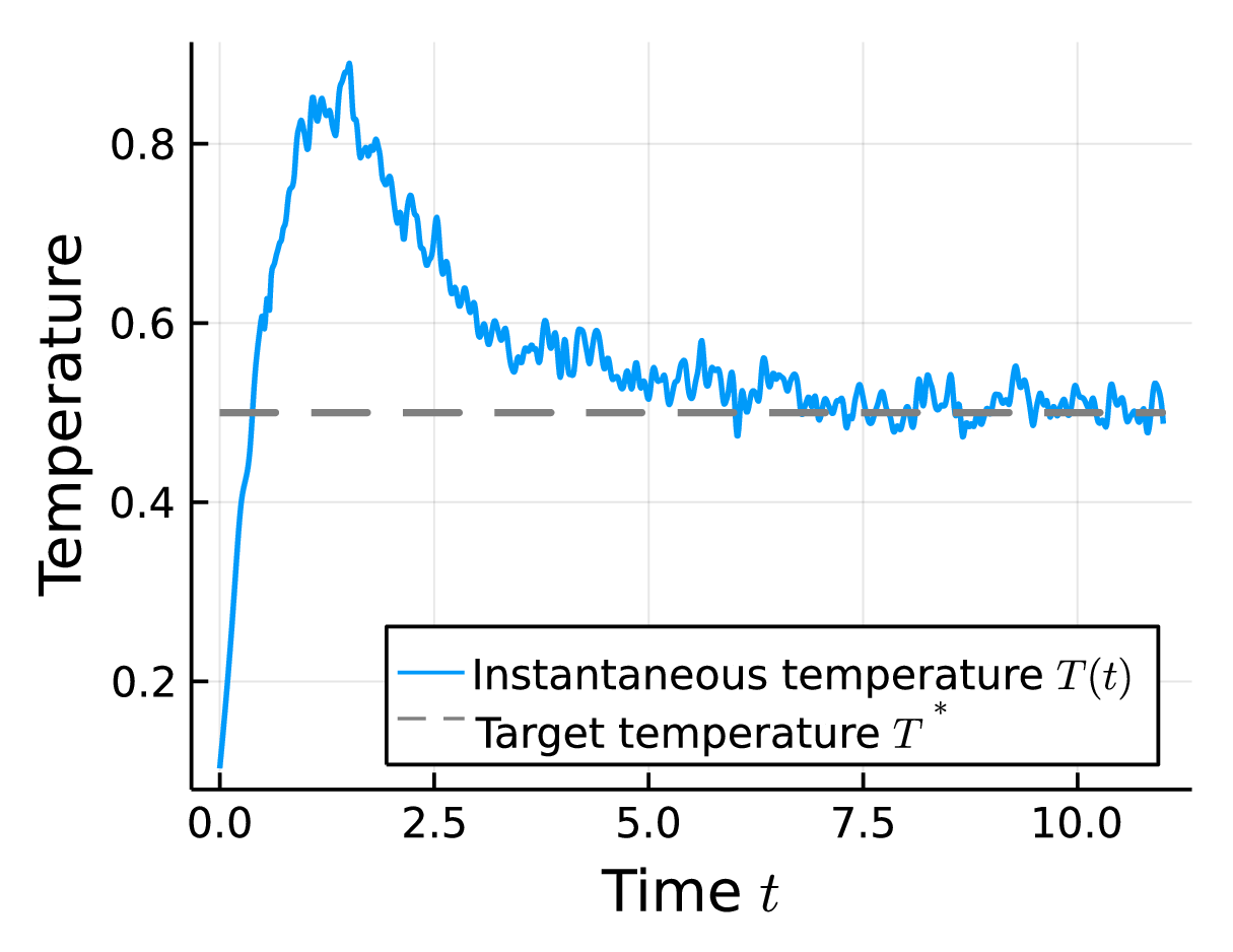
This procedure is carried out until the energy content of the system is adjusted to the desired temperature. An exemplary evolution of the instantaneous temperature of a system coupled to a bath at \(T^*=0.5\) modeled by the heat flux approach is shown in Fig. 4.
1.4.5 Link-cell trick
The computationally costly part of molecular dynamics simulations is determining the forces acting on the particles, because the positions of all other particles have to be considered to compute \(F_i(\mathbf r(t))\). The complexity of this task is in general \(\mathcal O(N^2)\), meaning that the compute time grows quadratically with increasing number of particles. However, physical potentials typically decay with increasing distance and often allow to introduce a cutoff radius \(r_c\), as we did above for the Lennard-Jones potential. This means, that in those cases a particle does not interact with all other particles, but just with those that are close enough. This fact is exploited by the link-cell trick in order to reduce the cost of computing forces.
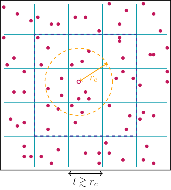
The idea of the link-cell trick is to identify particles that can interact with each other by dividing the simulation cube into smaller cells with a linear dimension \(\ell\) that is just slightly larger than \(r_c\), \(l\gtrsim r_c\). This is shown schematically in Fig. 5, where this time all particles are marked in red, because for this purpose we have to “project” all real particles into the same simulation cube. Now, we can create for each cell a list of all particles that are contained in it. The fact that interactions are restricted to distances smaller than \(r_c\) means that the forces of each particle are determined only by the other particles in the same cell and those in the eight neighboring cells, as indicated in Fig. 5. This means for the algorithm that we do not have to inspect all possible pairs of particles, but only those particles contained in neighboring boxes. This way, the link-cell trick allows us with a fixed particle density to increase the volume \(V\) of the simulation cube at a cost that is linear in \(V\) instead of the quadratic scaling that would result from the naive approach to compute the forces.
2 Preparation
2.1 Theory
While you familiarize yourself with the theoretical background, find answers to the following questions:
What could be a good cutoff distance \(r_c\) for the Lennard-Jones potential?
Derive the explicit formula to compute \(F_k(\mathbf r)\).
What are possible tests to verify the correct implementation of the computation of the forces and of the time integration?
2.2 Coding
For this project you will create your own implementation of a molecular dynamics simulation of the Lennard-Jones liquid.
When composing the simulation from scratch, the central building blocks that you need to implement are the following:
Write a function that computes the minimum image distance defined in Eq. 26 from given positions of two simulation particles.
Write a function that computes the force vector \(\mathbf F(\mathbf r)\) from the given particle positions \(\mathbf r\).
Write a function that performs the velocity Verlet integration step.
Write functions to compute all observables of interest from the phase space coordinates \((\mathbf p, \mathbf r)\).
Write a function that performs a binning analysis for a given sequence of observables \(O_i=O(\mathbf s^{(i)})\) following the instructions given on the toolbox page [3].
Optional: Consider implementing the link-cell trick described in Section 1.4.5 to be able to reach larger system sizes.
Before proceeding to the actual simulations, verify the correctness of your implementation with suited tests.
3 Tasks
Verify with a few examples that the heat flux approach leads to equilibration of the system at the target temperature. Can you verify that the parameters \(\tau_T\) determines the time scale for the approach to the desired temperature?
Perform the following tasks at two distinct points of the Lennard-Jones phase diagram, where you expect a gas or a liquid, respectively:
Confirm the equilibration of the system by comparing the observed velocities with the Maxwell-Boltzmann distribution.
Plot the two-particle distribution function \(g^{(2)}(r)\) and discuss its main features and differences between the two points. How does the finite volume of the simulation cube affect the results?
Compute the velocity autocorrelation function and confirm that its short-time dynamics can be obtained from \(g^{(2)}(r)\).
Compare the self-diffusion coefficient obtained from the velocity autocorrelation function with the one resulting from the squared distance.
Perform one simulation close to the Lennard-Jones critical point \((\rho_c,T_c)\approx(0.31,1.26)\) in order to
determine the pressure at the critical point of the Argon liquid. Compare your result to a value given in the literature, e.g. https://webbook.nist.gov/cgi/inchi?ID=C7440371&Mask=4#Thermo-Phase.