Quantum circuits
1 Theory
1.1 Introduction
The construction of a practically useful quantum computer is a long standing scientific quest. Although the underlying idea to build a computer based on the principles of quantum mechanics dates back to the early 1980s, building and programming quantum computers is a significant challenge due to the fragile nature of qubits and the difficulty in controlling them. Nevertheless, recent advances in hardware and software have led to the development of small-scale quantum computers with which solving proof-of-principle problems has become feasible despite the remaining imperfections. Notably, it has been claimed that some of the experiments already prove “quantum advantage”, meaning that the problem solved would be unfeasible on a classical computer.
The substantial interest that quantum computing currently draws from academics, politics, and industry is rooted in the fact that a universal fault-tolerant quantum computer – should it become available in the future – could revolutionize the fields of cryptography, chemistry, and materials science, among others. Most popular is the example of Shor’s algorithm that would allow us to factor primes in polylogarithmic time on a quantum computer, thereby breaking the foundation of modern cryptographic schemes that rely on the classically unfeasible complexity of the problem. While Shor’s algorithm would require a genuinely fault-tolerant quantum computer, applications in chemistry and physics that exploit the fact that a quantum computer follows precisely the laws of physics that one aims to study to speed up simulations. This was, in fact, Richard Feynmans early vision for the quantum computer, expressed in his famous quote “Nature isn’t classical, dammit, and if you want to make a simulation of nature, you’d better make it quantum mechanical, …”.
Quantum circuits are at the heart of a universal model of quantum computation. But they are also of interest from viewpoints beyond the pure quantum information perspective. The central objective of this lab course project is to implement a quantum circuit emulator on your classical computer. Following Feynman’s proposal, you will use your emulator to explore a cirquit-based simulation of quantum many-body dynamics, which is, in fact, simultaneously among the most efficient ways to numerically simulate quantum dynamics. But your emulator will not be restricted to this single use case. As an optional part of the project, you can for example continue to investigate the limits of classical computation by mimicking Google’s toy problem for the demonstration of “quantum advantage”.
1.2 Recap: Quantum mechanics of composite systems
In the following, we briefly review some basics of quantum mechanics. For a more comprehensive presentation you can refer to any quantum mechanics text book; one resource that could be particularly useful in the context of this project is Ref. [1].
The simplest possible quantum system is a two-level system whose Hilbert space of states is spanned by two orthogonal basis states \(|{0}\rangle\) and \(|{1}\rangle\), \(\mathcal H=\text{span}\{|{0}\rangle,|{1}\rangle\}=\mathbb C^2\). Let us consider a quantum system that is composed of two such two-level systems \(A\) and \(B\). The composite Hilbert space is the tensor product of the two elementary Hilbert spaces, \(\mathcal H_{AB}=\mathcal H_A\otimes\mathcal H_B\), meaning a possible choice for an orthogonal basis is \(\{|{0}\rangle_A\otimes|{0}\rangle_B,|{0}\rangle_A\otimes|{1}\rangle_B,|{1}\rangle_A\otimes|{0}\rangle_B,|{1}\rangle_A\otimes|{1}\rangle_B\}\). In the following, we will abbreviate this notation via the convention \(|{ab}\rangle\equiv|{a}\rangle_A\otimes|{b}\rangle_B\). This construction immediately generalizes to systems that are composed of more than two parts and from the combinatorial construction of the canonical orthogonal basis it is clear that the dimension of the total Hilbert space grows exponentially with the number of components.
The matrices \[\begin{aligned} \mathbb 1=\begin{pmatrix}1&0\\0&1\end{pmatrix}\ ,\quad \hat X=\begin{pmatrix}0&1\\1&0\end{pmatrix}\ ,\quad \hat Y=\begin{pmatrix}0&-i\\i&0\end{pmatrix}\ ,\quad \hat Z=\begin{pmatrix}1&0\\0&-1\end{pmatrix} \end{aligned}\qquad{(1)}\] form a basis of the space of Hermitian operators acting on the two level Hilbert space \(\mathbb C^2\), meaning that any physical observable can be constructed as a linear combination of the four. Arbitrary operators acting on Hilbert spaces of composite systems are obtained from these as tensor products, for example the \(\hat X\)-operator acting on the first factor and the \(\hat Z\)-operator acting on the second factor, \[\begin{aligned} \hat X\otimes\hat Z= \begin{pmatrix} X_{00}Z_{00}&X_{00}Z_{01}&X_{01}Z_{00}&X_{01}Z_{01}\\ X_{00}Z_{10}&X_{00}Z_{11}&X_{01}Z_{10}&X_{01}Z_{11}\\ X_{10}Z_{00}&X_{10}Z_{01}&X_{11}Z_{00}&X_{11}Z_{01}\\ X_{10}Z_{10}&X_{10}Z_{11}&X_{11}Z_{10}&X_{11}Z_{11} \end{pmatrix} = \begin{pmatrix} 0&0&1&0\\ 0&0&0&-1\\ 1&0&0&0\\ 0&-1&0&0\\ \end{pmatrix}\ . \end{aligned}\qquad{(2)}\] In the expression above \(X_{ij}=\langle{i|\hat X|j}\rangle\) and \(Z_{ij}=\langle{i|\hat Z|j}\rangle\) denote the matrix elements of the Pauli operators and you can see that the tensor product corresponds to a block structure in the matrix representation.
A distinct physical phenomenon of composite quantum systems is the entanglement between different parts. Entangled systems can exhibit quantum correlations that violate bounds for correlation functions derived under the assumption of “local realism”, which demonstrates that classical theories cannot describe these phenomena. How strongly two parts \(A\) and \(B\) of a composite system are entangled for a given state \(|{\psi}\rangle\) is quantified by the entanglement entropy \[\begin{aligned} S_A=-\text{tr}\big(\rho_A\ln\rho_A\big)=-\text{tr}\big(\rho_B\ln\rho_B\big)=S_B\ . \end{aligned}\qquad{(3)}\] Here, \(\text{tr}(\cdot)\) denotes the trace and \(\rho_A\) is the reduced density matrix of subsystem \(A\), which is defined as \[\begin{aligned} \rho_A=\text{tr}_B\big(|{\psi}\rangle\langle{\psi}|\big)=\sum_{b=1}^{\text{dim}(\mathcal H_B)}\big(\mathbb 1_A\otimes\langle{b}|_B\big)\ |{\psi}\rangle\langle{\psi}|\ \big(\mathbb 1_A\otimes|{b}\rangle_B\big)\ . \end{aligned}\qquad{(4)}\] This expression defines the partial trace over subsystem \(B\), \(\text{tr}_B(\cdot)\), and the reduced density matrix \(\rho_B\) is defined analogously. The entanglement entropy vanishes for product states \(|{\psi}\rangle=|{\psi_A}\rangle\otimes|{\psi_B}\rangle\), where both subsystems are uncorrelated. For maximally entangled states, the entanglement entropy reaches the maximal possible value \(S_A=\ln(\text{dim}(\mathcal H_A))\).
1.3 Qubits and quantum circuits
In classical computation the minimal unit of information is a bit, i.e., a binary variable. The central idea of quantum computing is to replace the bit by a qubit, i.e., a normalized vector in \(\mathbb C^2\), which is the mathematical description of the physical state of a quantum mechanical two-level system. According to the rules of quantum mechanics, the state of a quantum register holding \(N\) qubits is then described by a normalized vector in \(\mathbb C^{2^N}\).
The physical implementation of a quantum register that is well isolated from its environment will evolve according to the Schrödinger equation governed by a Hamiltonian operator that describes the mutual interactions between the qubits and, additionally, external control fields. This means that the time evolution of the register from time \(t_1\) to time \(t_2\) is fully determined by a unitary time evolution operator \(\hat U(t_2,t_1)\). Therefore, it is most natural and, in fact, most general to assume that quantum information processing means applying unitary transformations to the state of the quantum register. Since the unitary operations include the logical operations of classical reversible computation, it is standing in reason to consider their generalization as starting points for quantum computation. Below, we will exemplarily introduce the quantum versions of some elementary classical one- and two-bit gates. Moreover, we will introduce a graphical notation for unitary transformations that will allow us to visualize the composition of quantum algorithms in the form of quantum circuits.
1.3.1 Single qubit operations
A first example of a single-qubit operation is the generalization of the classical negation, which for \(b'=\text{NOT}(b)\) follows the truth table
| b | b’ |
|---|---|
| 0 | 1 |
| 1 | 0 |
The generalization to the quantum case is the unitary that maps \(|{0}\rangle\mapsto|{1}\rangle\) and \(|{1}\rangle\mapsto|{0}\rangle\), i.e. the Pauli-X operator \[\begin{aligned} \hat X=\begin{pmatrix}0&1\\1&0\end{pmatrix}\ . \end{aligned}\qquad{(5)}\] When considering a register of \(N\) qubits, we have to specify in addition which qubit the operator acts on and we introduce the short notation \[\begin{aligned} \hat X^{(i)}=\mathbb 1_1\otimes\ldots\otimes\mathbb 1_{i-1}\otimes \hat X\otimes\mathbb 1_{i+1}\otimes\ldots\otimes\mathbb 1_N\ . \end{aligned}\qquad{(6)}\]
More generally, the model of quantum circuits allows us to act with arbitrary unitary operations on a single qubit. One possible parameterization of general single qubit unitaries is given by \[\begin{aligned} \hat U(\alpha,\beta,\gamma,\delta)= e^{i\alpha} \begin{pmatrix} e^{-i\frac{\beta+\delta}{2}}\cos\frac{\gamma}{2}& e^{-i\frac{\beta-\delta}{2}}\sin\frac{\gamma}{2}\\ -e^{i\frac{\beta-\delta}{2}}\sin\frac{\gamma}{2}& e^{i\frac{\beta+\delta}{2}}\cos\frac{\gamma}{2} \end{pmatrix} = e^{i\alpha}\hat R_{\hat z}(\beta)\hat R_{\hat y}(\gamma)\hat R_{\hat z}(\delta)\ , \end{aligned}\qquad{(7)}\] where \[\begin{aligned} \hat R_{\hat n}(\theta)=\exp\Big[-i\frac{\theta}{2}\big(n_x\hat X+n_y\hat Y+n_z\hat Z\big)\Big] \end{aligned}\qquad{(8)}\] denotes a rotation around the axis \(\hat n=(n_x,n_y,n_z)\) by an angle \(\theta\).
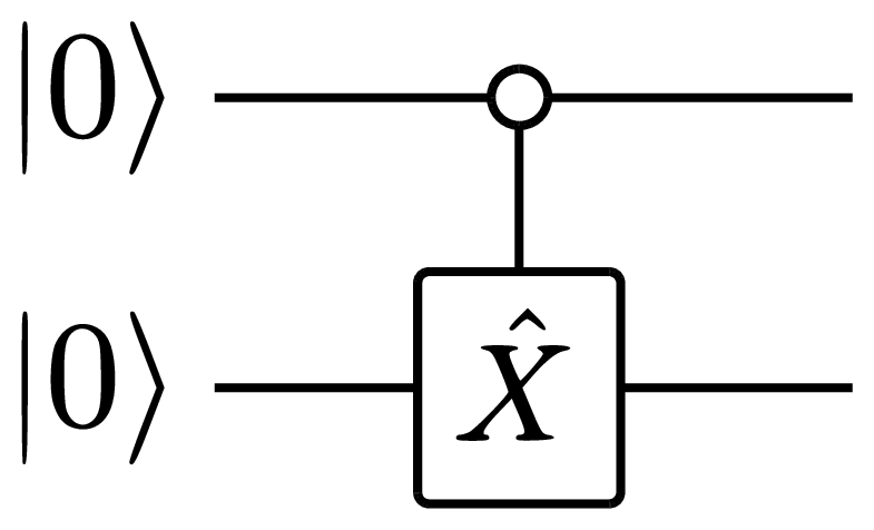
For the following, it will be useful to introduce a graphical notation for the action of unitary operations on qubits. An \(X\)-gate acting on a single qubit that is initially in state \(|{0}\rangle\) is represented as
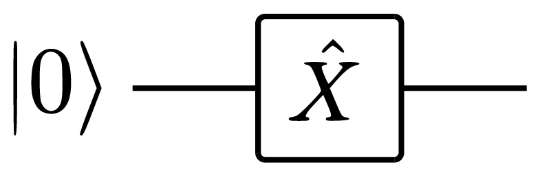
In this diagram the horizontal line represents the time line of the qubit, and time progresses from left to right. The box that is placed on this line represents the \(X\)-gate acting on the qubit.
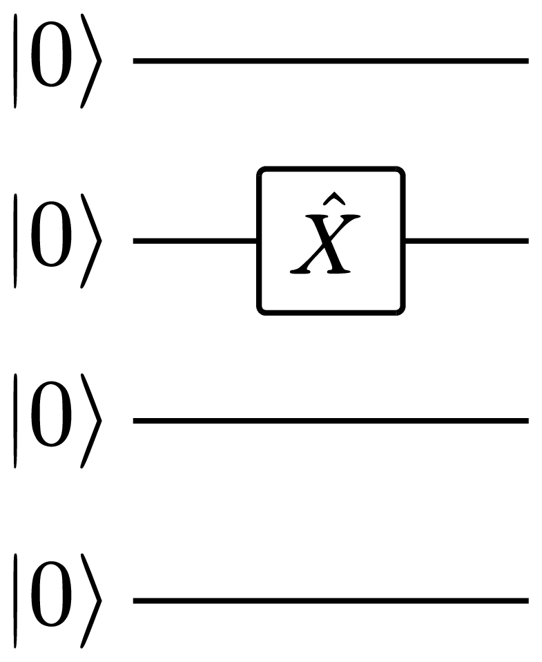
If we have multiple qubits in the register, say \(N=4\) for concreteness, the single qubit operation acting on qubit \(i=2\) is represented by
For fault tolerant general purpose quantum computing it is essential that arbitrary unitary operations on a register of qubits can be composed using only a small set of elementary gates. A first step in this direction is to realize that arbitrary single-qubit
1.3.2 Two-qubit operations
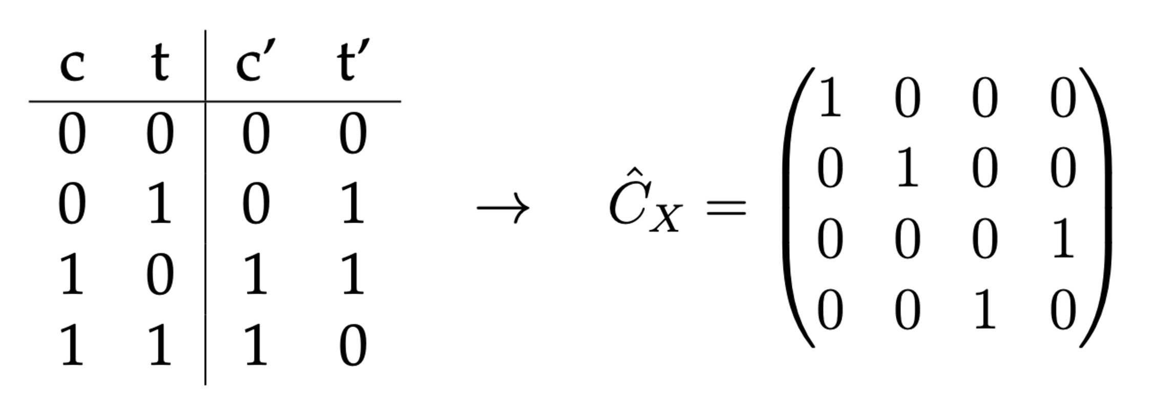
One example of a two bit operation is the controlled-not gate (CNOT), which flips the target bit \(t\) if the control bit \(c\) is in state 1. The generalization to the quantum version is obtained by translating the classical truth table to the action of the operation on the quantum computational basis states:
The graphical notation of the \(\hat C_X\) gate is given by
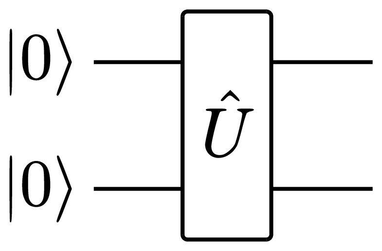
Here, the small empty circle is placed on time line of the control qubit, whereas the box with the \(\hat X\) operator is placed on the target qubit line. The connection between the two indicates that this is an operation that involves both qubits at the same time. This notation is, however, specific for the \(\hat C_X\) gate. General two qubit unitaries \(\hat U\) are denoted by boxes that connect to both involved qubit lines:
In analogy to classical computation, where arbitrary algorithms can be composed from a set of elementary logical gates that act on one or two bits at a time, arbitrary quantum algorithms can be composed from sequences of unitary operations that act non-trivially only on one or two qubits at a time. In fact, one can prove that any unitary operation on a set of qubits can be decomposed into a suited sequence of single qubit rotations (Eq. 8) and CNOT operations [1]. In Section 1.6 we will discuss how one- and two-qubit gates can be implemented for numerical simulations, which will be the basis for your efficient quantum circuit emulator.
1.3.3 Measurement
Through the application of a quantum circuit, the register of qubits is prepared in a specific superposition of the computational basis states, \(|{\psi}\rangle=\sum_{\mathbf b}\psi(\mathbf b)|{\mathbf b}\rangle\). In order for an algorithm to be useful, one has to be able to extract information from these quantum many-body states. This is achieved via projective measurements in the computational basis. Consider the projector \(\hat P_{\mathbf b}=|\mathbf b\rangle\langle\mathbf b|\) onto the computational basis state \(|{\mathbf b}\rangle\). Then, the probability of finding the measurement outcome \(\mathbf b\) is given by \[\begin{aligned} \mathcal P(\mathbf b)=\langle{\psi|\hat P_{\mathbf b}|\psi}\rangle=|\psi(\mathbf b)|^2\ . \end{aligned}\qquad{(9)}\] According to the rules of quantum mechanics, the observation of the measurement outcome \(\mathbf b\) updates our knowledge about the state of the system and as a consequence we have to project the wave function onto the respective basis state, \[\begin{aligned} |{\psi'}\rangle=\frac{1}{\sqrt{\mathcal P(\mathbf b)}}\hat P_{\mathbf b}|{\psi}\rangle\ . \end{aligned}\qquad{(10)}\] The information encoded in \(|{\psi}\rangle\) will, however, typically be more than what we learn by drawing a single sample from \(\mathcal P(\mathbf b)\). The usual approach is to draw a finite sample \(\mathcal M_{|{\psi}\rangle}=\{\mathbf b^{(n)}\}\) with \(\mathbf b^{(n)}\sim\mathcal P(\mathbf b)\). To obtain such a sample, the circuit has to be executed once for each element \(\mathbf b^{(n)}\). Each run means to initialize the register to \(\bigotimes_{i}|{0}\rangle\), apply the unitary circuit, and finally obtain one projective measurement outcome \(\mathbf b^{(n)}\) that can be added to the sample.
The sample \(\mathcal M_{|{\psi}\rangle}\) can then be used to compute all kinds of statistics one is interested in. For example, the expectation value of operators can be estimated via empirical means. Consider, for example, the Pauli-\(\hat Z\) operator acting on qubit \(i\). Since \(\hat Z\) is diagonal in the computational basis, we get \[\begin{aligned} \langle{\psi|\hat Z^{(i)}|\psi}\rangle=\sum_{\mathbf b}\langle{\mathbf b|\hat Z^{(i)}|\mathbf b}\rangle=\sum_{\mathbf b}\mathcal P(\mathbf b)(1+2b_i)\approx\frac{1}{|\mathcal M_{|{\psi}\rangle}|}\sum_{\mathbf b\in\mathcal M_{|{\psi}\rangle}}(1+2b_i)\ . \end{aligned}\qquad{(11)}\] In order to compute expectation values of operators that are not diagonal in the computational basis, one has to relate them to the Pauli-\(\hat Z\) operator via rotations. For example \[\begin{aligned} \langle{\psi|\hat X^{(i)}|\psi}\rangle =\langle{\psi|\hat R_{\hat y}^{(i)}(\pi/2)^\dagger\hat Z^{(i)}\hat R_{\hat y}^{(i)}(\pi/2)|\psi}\rangle\ . \end{aligned}\qquad{(12)}\] The rotation can formally be absorbed into the quantum circuit as one additional layer of gates.
A significant error source on current quantum computers are faulty measurement outcomes – so-called readout errors. Due to the technical implementation, there is often a tendency to mis-interpret the actual measurement outcome 1 as 0 for individual qubits. This means that in collecting observations for the sample \(\mathcal M_{|{\psi}\rangle}\), a configuration \(\tilde{\mathbf b}\) is registered instead of \(\mathbf b\), where \(\tilde b_i=b_i\) except for some \(b_j=1\) where one gets \(\tilde b_j=0\). This mis-interpretation happens independently for each qubit with a probability \(p_{\text{err}}\).
1.4 Digital quantum simulation
As already mentioned in Section 1.1, the simulation of many-body quantum systems is one of the potential use cases of quantum computing. We will for our discussion consider physical systems that are composed of spin-1/2 degrees of freedom, because the two states of the spin-1/2 can immediately be mapped to the two states of a qubit. But this is by no means a general restriction of quantum simulation.
In this section we will first discuss a general approach to simulate quantum many-body systems on a classical computer, before turning to a cirquit model of quantum dynamics that is applicable on digital quantum computers and simultaneously constitutes the basis for one of the most efficient numerical time evolution methods for classical computers.
1.4.1 Full basis simulations of many-body quantum systems
The straightforward starting point to classically simulate a system of \(N\) spin-1/2 degrees of freedom is to store all coefficients of the state vector \(|{\psi}\rangle\in\mathbb C^{2^N}\) in memory. For this purpose one has to select a computational basis, and a typical choice is the basis of mutual eigenstates of all \(\hat Z^{(i)}\) operators. The basis states are denoted as \(|{b_1\ldots b_N}\rangle\), where \(b_i\in\{0,1\}\) such that \(\hat Z^{(i)}|{b_1\ldots b_N}\rangle=(1-2b_i)|{b_1\ldots b_N}\rangle\). The object stored in memory is then an array of the form \[\begin{aligned} \boldsymbol{\Psi}=\big[\langle{0\ldots 00|\psi}\rangle,\langle{0\ldots 01|\psi}\rangle,\langle{0\ldots 10|\psi}\rangle,\ldots,\langle{1\ldots 11|\psi}\rangle\big] \end{aligned}\qquad{(13)}\] and, clearly, the amount of memory required is proportional to the Hilbert space dimension \(\text{dim}(\mathcal H)=2^N\), which is equal to the number of different bit-strings of length \(N\).
Notice that the basis state labels simultaneously enumerate the wave function coefficients. When regarding the bit strings as binary numbers, we can use the integer \(n=\texttt{decimal}(b_1\ldots b_N)\) to enumerate \(\Psi_n\) – the entries of the array of wave function coefficients \(\boldsymbol\Psi\). Alternatively, we can view \(\boldsymbol\Psi\) as a tensor of rank \(N\) with entries \(\psi_{b_1,\ldots,b_N}\). In the latter case \((b_1,\ldots,b_N)\) is the multi-index of the stored coefficients and it can be obtained for a given \(n\) as \(b_1\ldots b_N=\texttt{binary}(n)\). We will in the following use \(n\) or \((b_1,\ldots,b_N)\) exchangeably as indices of the basis states, for example, \(|{n}\rangle\equiv|{b_1\ldots b_N}\rangle\) or \(\Psi_n\equiv\Psi_{b_1,\ldots,b_N}\).
As we are considering discrete degrees of freedom, the action of a physical operator \(\hat O\) on the quantum state \(|{\psi}\rangle\) corresponds to a matrix-vector product: \[\begin{aligned} \hat O|{\psi}\rangle=\sum_{n=0}^{2^N-1}\sum_{n'=0}^{2^N-1}O_{n,n'}\langle{n'|\psi}\rangle|{n}\rangle \end{aligned}\qquad{(14)}\] Here, we introduced the matrix elements of \(\hat O\), \[\begin{aligned} O_{n,n'}\equiv O_{(b_1,\ldots,b_N),(b_1',\ldots,b_N')}=\langle{b_1,\ldots,b_N|\hat O|b_1',\ldots,b_N'}\rangle\ . \end{aligned}\qquad{(15)}\] Consider, for example, the operator \(\hat X^{(i)}\). Due to the tensor product structure in Eq. 6, its matrix elements are given by \[\begin{aligned} X^{(i)}_{(b_1,\ldots,b_N),(b_1',\ldots,b_N')}= \delta_{b_i,1-b_i'}\prod_{j\neq i}\delta_{b_j,b_j'}\ , \end{aligned}\qquad{(16)}\] where \(\delta_{i,j}\) denotes the Kronecker-Delta. As another example, consider the CNOT gate defined in Section 1.3.2, acting on qubits \(i\) and \(j\). The matrix elements are \[\begin{aligned} \big[C_X^{(i,j)}\big]_{(b_1,\ldots,b_N),(b_1',\ldots,b_N')}=\big(\delta_{b_i,0}\delta_{b_j,b_j'}+\delta_{b_i,1}\delta_{b_j,1-b_j'}\big)\prod_{k\neq i,j}\delta_{b_k,b_k'}\ . \end{aligned}\qquad{(17)}\] A naive approach to represent such operators for the purpose of a simulation would be to store the corresponding matrices in memory. The size of the required memory would be \(\mathcal O(2^{2N})\), i.e., scaling quadratically with the Hilbert space dimension. However, the two examples above already reveal a typical feature of physical operators, namely sparseness in the computational basis: Only a tiny fraction of the \(2^{2N}\) matrix elements is non-vanishing. This structure can be exploited for more efficient simulations, as we will discuss below.
Let us for now assume that for an operator \(\hat O\) we can implement a representation \(\bar O\) in our simulation that allows us to compute \(|{\phi}\rangle=\hat O|{\psi}\rangle\) as \[\begin{aligned} \boldsymbol\Phi=\bar O\boldsymbol\Psi \end{aligned}\qquad{(18)}\] such that \[\begin{aligned} \Phi_{b_1,\ldots,b_N}=\sum_{(b_1',\ldots,b_N')\in\{0,1\}^N}O_{(b_1,\ldots,b_N),(b_1',\ldots,b_N')}\Psi_{b_1',\ldots,b_N'} \end{aligned}\qquad{(19)}\] as prescribed by Eq. 14. This does not only allow us to evaluate the action of the operator on a quantum state; we can also use the result to compute the expectation value of the operator, \[\begin{aligned} \langle{\psi|\hat O|\psi}\rangle=\boldsymbol\Phi\cdot\boldsymbol\Psi=\sum_n\Phi_n^*\Psi_n\ , \end{aligned}\qquad{(20)}\] a typical quantity of interest.
The limitation of the approach outlined in this section is clearly the exponential growth of the Hilbert space dimension with the number of degrees of freedom – the quantum curse of dimensionality. When no additional structure can be exploited to reduce the dimensionality the largest feasible system sizes on today’s most powerful supercomputers are about \(N\approx50\). The central idea of digital quantum simulation is to exploit the fact that the state space of a qubit register is already quantum mechanical. In the following, we discuss how to formulate the solution of the time-dependent Schrödinger equation in terms of a quantum circuit. This would allow us to use a quantum computer for the simulation, but it also reveals that in a classical simulation the largest objects that have to be stored in memory have size of \(\mathcal O(2^N)\) instead of \(\mathcal O(2^{2N})\) that could be naively expected for example for operators, cf. Eq. 15.
1.4.2 A circuit model of quantum dynamics
Within this project you will simulate the dynamics of a quantum many-body system that is well isolated from its environment. This means that its evolution is prescribed by the time-dependent Schrödinger equation \[\begin{aligned} i\frac{d}{dt}|{\psi}\rangle=\hat H|{\psi}\rangle\ , \end{aligned}\qquad{(21)}\] where the Hamiltonian operator \(\hat H\) describes the interactions within the system and the effect of external fields applied to it. The model that we will be interested in is the quantum Ising chain of spin-1/2 particles, subject to an external magnetic field. It is described by \[\begin{aligned} \hat H=-J\sum_{i=1}^L\hat Z^{(i)}\hat Z^{(i+1)}-h_z\sum_{i=1}^L\hat Z^{(i)}-h_x\sum_{i=1}^L\hat X^{(i)} \end{aligned}\qquad{(22)}\] Here, \(h_{x/z}\) are the \(x\)- and \(z\)-components of the magnetic field and \(J\) is the strength of the Ising coupling. Moreover, we assume periodic boundary conditions, i.e., \(\hat Z^{(L+1)}\equiv\hat Z^{(1)}\).
For a given initial state \(|{\psi_0}\rangle\) the formal solution of the Schrödinger equation is given by \[\begin{aligned} |{\psi(t)}\rangle=e^{-i\hat Ht}|{\psi_0}\rangle\equiv\hat U(t)|{\psi_0}\rangle\ . \end{aligned}\qquad{(23)}\] Here, we introduced the time evolution operator \(\hat U(t)=e^{-i\hat Ht}\), which is a unitary operator. Since we learned above that arbitrary unitaries can be composed as circuits of elementary few-qubit unitaries, our aim is now to decompose \(\hat U(t)\) accordingly. This decomposition will be the basis for the efficient implementation of a numerical simulation, and it is at the same time a viable route for the envisioned simulation of quantum dynamics on an actual quantum computer. For this purpose, we employ a Suzuki-Trotter decomposition of the time evolution operator.
A straightforward approach to simulate this time evolution would be to work with an explicit matrix representation of \(\hat U(t)\). This, however, requires the exponentiation of the Hamiltonian matrix, which has a cost cubic in the Hilbert space dimension (cf. Section 1.6.3), which, in turn, grows exponentially with the number of degrees of freedom. Since we learned above that a quantum computer allows us to compose arbitrary unitaries as circuits of elementary few-qubit unitaries, our aim is now to decompose \(\hat U(t)\) accordingly.
Consider two non-commuting operators \(\hat A\) and \(\hat B\). Then, the their exponentiated sum for a small time step \(\delta\) can be approximately decomposed as \[\begin{aligned} e^{-i\delta(\hat A+\hat B)}=e^{-i\delta \hat A}e^{-i\delta \hat B}+\mathcal O(\delta^2)\ , \end{aligned}\qquad{(24)}\] which can be checked by expanding the exponentials. Approximating \(e^{-i\delta(\hat A+\hat B)}\approx e^{-i\delta \hat A}e^{-i\delta \hat B}\) is called a first order Suzuki-Trotter decomposition. In fact, one can easily obtain a higher accuracy through a small modification, \[\begin{aligned} e^{-i\delta(\hat A+\hat B)}=e^{-i\frac\delta2 \hat B}e^{-i\delta \hat A}e^{-i\frac\delta2 \hat B}+\mathcal O(\delta^3)\ , \end{aligned}\qquad{(25)}\] which yields the second order Suzuki-Trotter decomposition.
To apply the Suzuki-Trotter decomposition to our concrete problem, we can split the Hamiltonian 22 into \[\begin{aligned} \hat A=-J\sum_{i}\hat Z^{(i)}\hat Z^{(i+1)}-h_z\sum_{i}\hat Z^{(i)} \end{aligned}\qquad{(26)}\] and \[\begin{aligned} \hat B=-h_x\sum_{i}\hat X^{(i)}\ . \end{aligned}\qquad{(27)}\] Then, both \(\hat A\) and \(\hat B\) consist only of sums of mutually commuting operators. This is important for our goal to rewrite \(\hat U(t)\) as a circuit of few-qubit unitaries, because it means that \[\begin{aligned} e^{-i\Delta t\hat A}=e^{-i\Delta t(-J\sum_{i}\hat Z^{(i)}\hat Z^{(i+1)}-h_z\sum_{i}\hat Z^{(i)})} =\prod_ie^{-i\Delta t(-J\hat Z^{(i)}\hat Z^{(i+1)}-h_z\hat Z^{(i)})} \end{aligned}\qquad{(28)}\] and \[\begin{aligned} e^{-i\Delta t\hat B}=e^{-i\Delta t(-h_x\sum_{i}\hat X^{(i)})} =\prod_ie^{-i\Delta t(-h_x\hat X^{(i)})}\ . \end{aligned}\qquad{(29)}\] Thereby, we further decomposed the two Suzuki-Trotter factors into sequences of gates that act on no more than two qubits at a time. In the graphical notation, we can write
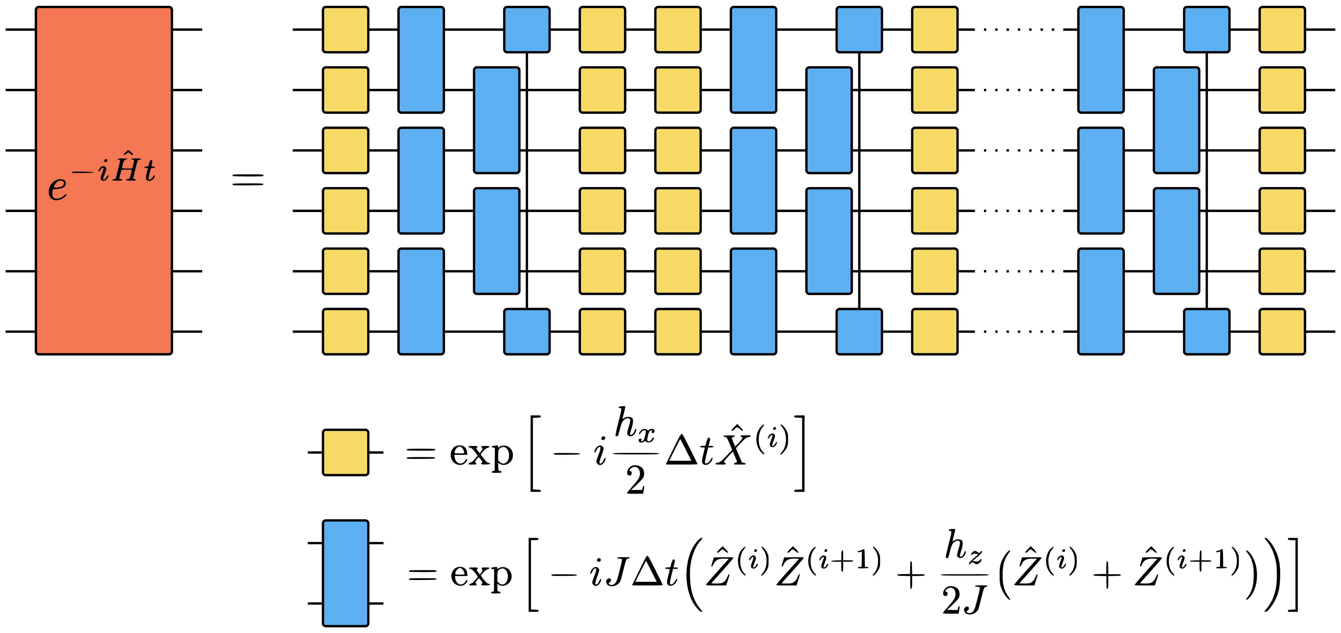
This means, that we can use circuits of the form given above to approximate, for a small enough time step \(\Delta t=\frac{t}{n}\), the time evolution operator \[\begin{aligned} \hat U(t)=\Big(e^{-i\hat H\Delta t}\Big)^n \end{aligned}\qquad{(30)}\] for the quantum Ising model.
A straightforward approach to simulate this time evolution on a classical computer would be to work with an explicit matrix representation of \(\hat U(t)\). This, however, requires the exponentiation of the Hamiltonian matrix, which has a cost of \(\mathcal O(2^{3N})\), i.e., cubic in the Hilbert space dimension (cf. Section 1.6.3). In Section 1.6.1 we will discuss that using the Suzuki-Trotter circuit model reduces the cost to \(\mathcal O(2^{N})\), which – although still exponential in the system size – is a substantial improvement. The cost of performing a Trotter-Suzuki time step on a quantum computer is linear in the number of degrees of freedom. Therefore, this circuit-based quantum time evolution would be of substantial interest if a quantum computer with more than 50 qubits and sufficiently long coherence times became available. The same principle can be applied to systems with more practical relevance, for example in quantum chemistry.
Since the presently available qubit numbers and coherence times are, however, limited, one needs to consider even better tailored problems in order to demonstrate “quantum advantage”, i.e., the ability of existing quantum computers to solve a classically unfeasible task. In the following section we will discuss an experiment that was recently conducted by Google on their superconducting quantum processor as a first demonstration of “quantum advantage”.
1.5 Random circuit sampling – optional
Thanks to remarkable progress over the past two decades, various forms of quantum processors are available today across the world. The qubit numbers and coherence times are still clearly limited, but the exploration of these platforms for a large variety of use cases is an active research direction. Nonetheless, all tasks of practical relevance that a quantum computer could be useful for remained so far out of reach. In order to still demonstrate that quantum computers can solve tasks that are virtually impossible for any conceivable classical computer with current quantum devices, one therefore has to resort to tailored problems that suit the presently available capabilities. One example of such a tailored problem is random circuit sampling, which we will discuss in this section. This problem has been devised by researchers at Google to demonstrate that their superconducting quantum processor already achieves “quantum supremacy” over classical computers [2].
1.5.1 Random quantum circuits
A random quantum circuit is composed from randomly chosen quantum gates. The circuit used in the “quantum supremacy” experiment has the following form:
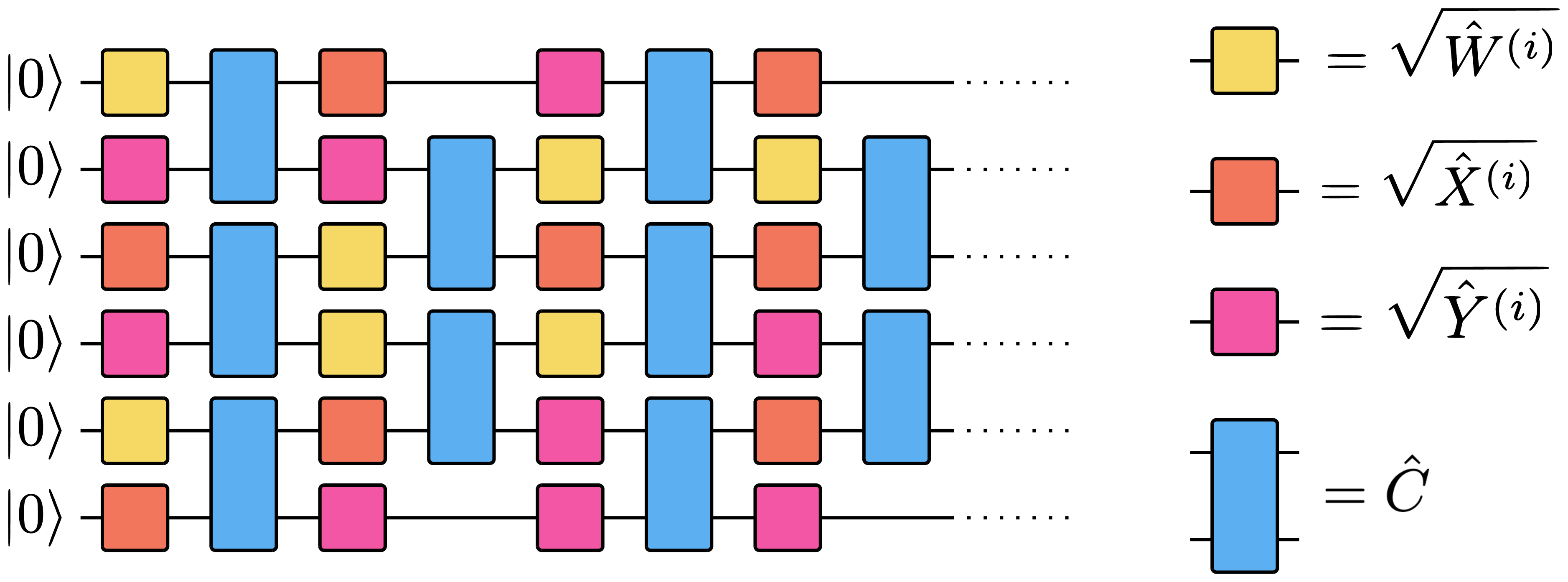
The random component in this circuit is the placement of single qubit gates, which are randomly drawn from the set \(\{\sqrt{\hat W},\sqrt{\hat X}, \sqrt{\hat Y}\}\). These gates are defined by \[\begin{aligned} \sqrt{\hat W}=\frac{1}{\sqrt2}\begin{pmatrix}1&-\sqrt{i}\\\sqrt{i}&1\end{pmatrix} \ ,\quad \sqrt{\hat X}=\frac{1}{\sqrt2}\begin{pmatrix}1&-i\\-i&1\end{pmatrix} \ ,\quad \sqrt{\hat Y}=\frac{1}{\sqrt2}\begin{pmatrix}1&-1\\1&1\end{pmatrix} \end{aligned}\qquad{(31)}\] The layers of randomly selected single qubit gates is interleaved by layers of two qubit gates. The qubit gate used is \[\begin{aligned} \hat C= \begin{pmatrix} 1&0&0&0\\ 0&0&-i&0\\ 0&-i&0&0\\ 0&0&0&e^{-i\pi/6} \end{pmatrix} \ . \end{aligned}\qquad{(32)}\] The placement of the two-qubit gates will in a real experiment depend on the layout of the quantum chip. On a superconducting quantum computer entangling operations can only be applied to neighboring qubits that are connected through some resonator. This means that any two qubit gate that acts on non-neighboring qubits have to be implemented by swapping the states of physical qubits until the computational qubit states of interest are located in neighboring physical qubits. This quickly renders the circuits very deep and impedes performance on current devices. Therefore, the circuits considered to demonstrate “quantum advantage” only work with entangling gates between physically neighboring quibts. Here, we are assuming a linear arrangement of the qubits. The \(\hat C\) gates are applied in an alternating fashion on the even and odd links between the qubits.
1.5.2 Random circuit sampling
As already mentioned in Section 1.3.3, information is extracted from a quantum computer by performing projective measurements of the individual qubits in the computational basis. By repeated execution of the quantum circuit a sample of bitstrings encoding the measurement outcomes is collected, for example, \[\begin{aligned} \mathcal M=\{0111001,10110011,\ldots\} \end{aligned}\qquad{(33)}\] In the limit of large sample sizes the relative frequency of bitstring \(\mathbf s\) to appear in \(\mathcal M\) is given by the Born probability \(|\psi(\mathbf s)|^2\). Now, one could expect, that \(|\psi(\mathbf s)|^2\) becomes a featureless uniform distribution for a random circuit. This is, however, not the case. Due to quantum interference within the given realization of the circuit, some bitstrings obtain a much larger probability than others. This fact is reflected in a theoretical result regarding the distribution of Born probabilities: At the end of a random circuit, the probability for a bitstring \(\mathbf s\) to have the Born probability \(|\psi(\mathbf s)|^2=p\) is \[\begin{aligned} \text{Pr}(p)=\kappa e^{-\kappa p}\ . \end{aligned}\qquad{(34)}\] Therefore, it is not trivial to sample bitstrings that follow the Born distribution generated by a given realization of a random circuit. In fact, the best known way of doing this on a classical computer is to simulate the circuit in order to obtain the wave function coefficients, the cost of which grows exponentially in the number of bits. By contrast, sampling this distribution on a quantum computer means executing the circuit and collecting the projective measurement outcomes. This requires linear resources in the bit-string length.
Clearly, the challenge remains to verify that the sampled bit-strings correspond to the desired distribution. If the wave function coefficients \(\psi(\mathbf b)\) and the corresponding Born probabilities \(\mathcal P(\mathbf b)\) are know, cross-entropy benchmarking (XEB) is one way of testing the obtained sample. For this purpose, one computes the linear XEB fidelity \[\begin{aligned} \mathcal F_{\text{XEB}}=2^N\big\langle\mathcal P\big(\mathbf b\big)\big\rangle_{\mathcal M}-1\ , \end{aligned}\qquad{(35)}\] where \(N\) is the number of qubits and \(\langle\mathcal P\big(\mathbf b\big)\rangle_{\mathcal M}=\frac{1}{\mathcal M}\sum_{\mathbf b\in\mathcal M}\mathcal P\big(\mathbf b\big)\) denotes the empirical mean over the sampled bit-strings. If the distribution that the bit-strings are sampled from equals \(\mathcal P\big(\mathbf b\big)\), \(\mathcal F_{\text{XEB}}=1\). If, however, the sampled bit-strings come from a uniform distribution, \(\mathcal F_{\text{XEB}}=0\). Any value between zero and one indicates that the distribution that has been sampled from has at least some similarity with the expected Porter-Thomas distribution.
The requirement of knowing the Born probabilities of course means that one needs to be able to compute them, for which one has to rely on a classical simulation of the circuit. In order to go beyond classically simulable qubit numbers, Google relied on a careful extrapolation of the XEB [2]. The aim of this project will not be to demonstrate quantum supremacy. Instead, you will explore the limitations of the classical emulation of quantum circuits and the effect of a typical imperfection of today’s devices, namely readout errors.
1.6 Efficient implementation of one- and two-qubit gates
The main objective of this project will be to implement a full basis simulator of quantum circuits based on the principles introduced in Section 1.4.1. Clearly, the exponential growth of the Hilbert space dimension imposes severe limitations on this approach, but for general quantum algorithms there are no known ways to circumvent this.1 In this section we will discuss an approach to at least render the treatment of quantum operators linear in the Hilbert space dimension instead of the naively quadratic or even cubic cost.
The starting point is the generalization of the examples given in Section 1.3 to arbitrary one- and two-qubit operations. Let us consider a single qubit operator \[\begin{aligned} \hat O=\begin{pmatrix}O_{0,0}&O_{0,1}\\O_{1,0}&O_{1,1}\end{pmatrix}\ . \end{aligned}\qquad{(36)}\] Then, it is straightforward to write the matrix elements of \(\hat O^{(i)}\) acting on the \(N\)-qubit Hilbert space: \[\begin{aligned} O^{(i)}_{(b_1,\ldots,b_N),(b_1',\ldots,b_N')}=O_{b_i,b_i'}\prod_{j\neq i}\delta_{b_j,b_j'} \end{aligned}\qquad{(37)}\] Similarly, for a two-qubit operator \[\begin{aligned} \hat O= \begin{pmatrix} O_{(00),(00)}&O_{(00),(01)}&O_{(00),(10)}&O_{(00),(11)}\\ O_{(01),(00)}&O_{(01),(01)}&O_{(01),(10)}&O_{(01),(11)}\\ O_{(10),(00)}&O_{(10),(01)}&O_{(10),(10)}&O_{(10),(11)}\\ O_{(11),(00)}&O_{(11),(01)}&O_{(11),(10)}&O_{(11),(11)} \end{pmatrix}\ . \end{aligned}\qquad{(38)}\] when acting on qubits \(i\) and \(j\), \[\begin{aligned} O^{(i,j)}_{(b_1,\ldots,b_N),(b_1',\ldots,b_N')}=O_{(b_i,b_j),(b_i',b_j')}\prod_{k\neq i,j}\delta_{b_k,b_k'}\ . \end{aligned}\qquad{(39)}\]
This structure can be exploited in two different ways, which we will explain in the following subsections. The third subsection below explains how to deal with the exponentiated operators resulting from the Suzuki-Trotter decomposition in Section 1.4.2.
1.6.1 Sparse operators
The matrices defined by Eqs. 37 and 39 are extremely sparse. For a given \((b_1,\ldots,b_N)\) there are at most two different multi-indices \((b_1',\ldots,b_N')\) with non-zero matrix element in the case of a single-qubit operator, and four of them for a two-qubit operator. This means that for the given matrix elements \(O_{b,b'}\) (or \(O_{(b_1,b_2),(b_1',b_2')}\)) the operator action defined in Eqs. 18 and 19 can be implemented as an on-the-fly operation. For example, one can implement a function that takes the matrix elements \(O_{b,b'}\) (or \(O_{(b_1,b_2),(b_1',b_2')}\)), the qubit index \(i\) (or indices \(i,j\)), and a multi-index \((b_1,\ldots,b_N)\) as input and returns a list of “connected” multi-indices \((b_1',\ldots,b_N')\) and corresponding non-vanishing matrix elements \(O^{(i,j)}_{(b_1,\ldots,b_N),(b_1',\ldots,b_N')}\). This allows one to sum up only the non-zero contributions in Eq. 19, rendering the computational cost linear in the Hilbert space dimension.
1.6.2 Tensor formalism
Let us consider the single qubit operation, from which the two-qubit case follows immediately. Inserting Eq. 39 into Eq. 19 yields \[\begin{aligned} \Phi_{b_1,\ldots,b_N} &=\sum_{(b_1',\ldots,b_N')\in\{0,1\}^N}O_{(b_1,\ldots,b_N),(b_1',\ldots,b_N')}^{(i,j)}\Psi_{b_1',\ldots,b_N'}\nonumber\\ &=\sum_{b_i\in\{0,1\}}O_{b_i,b_i'}\Psi_{b_1,\ldots,b_{i-1},b_i',b_{i+1},\ldots,b_N}\ . \end{aligned}\qquad{(40)}\] If we view \(\Psi_{b_1,\ldots,b_{i-1},b_i',b_{i+1},\ldots,b_N}\) as a rank-N tensor and \(O_{b_i,b_i'}\) as a rank-2 tensor (i.e., a matrix), the operation in the last row corresponds to a tensor contraction along the second axis of \(O\) and the \(i\)-th axis of \(\mathbf\Psi\). Such operations are implemented in the Julia and Python programming languages under the keyword “einstein summation” [3]. Therefore, an alternative approach to implement the operator action for a given operator \(\hat O\) acting non-trivially just on few qubits is the following:
Reshape the array \(\Psi_n\) of length \(2^N\) into a multi-dimensional array of shape \(2\times2\times\ldots\times2\) corresponding to \(\Psi_{b_1,\ldots,b_N}\).
Perform the tensor contraction (= Einstein summation) along the required axes to obtain the resulting state \(\Phi_{b_1,\ldots,b_N}\).
Reshape the multi-dimensional array \(\Phi_{b_1,\ldots,b_N}\) into a one dimensional array \(\Phi_n\), if required.
For this purpose, the graphical notation of the quantum circuit can again be useful. Considering, for example,
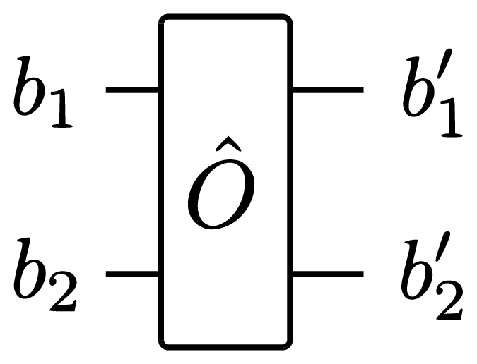
we can view the lines as the four indices of the matrix elements of the two-qubit operator. The qubit lines in a larger diagram can then be viewed as the individual qubit indices of the quantum state viewed as a rank-\(N\) tensor. And whenever the qubit lines are linked to an operator, it means that we have to perform a contraction along the corresponding axes.
1.6.3 Operator exponentiation
The few qubit gates resulting from the Suzuki-Trotter decomposition
introduced in Section 1.4.2 are defined as the
exponential of some given few qubit gates. Let us consider the gate
\[\begin{aligned}
\hat G^{(i)}=e^{-i\Delta t\hat X^{(i)}}
\end{aligned}\qquad{(41)}\] as an example. The first step
to perform the exponentiation is to find an eigendecomposition of the
single qubit matrix \(X\), i.e., a
unitary \(\hat V\) and a diagonal
matrix \(\Lambda\) containing the
eigenvalues \(\lambda_1,\lambda_2\)
such that \[\begin{aligned}
\hat X=\hat V\Lambda \hat V^\dagger\ .
\end{aligned}\qquad{(42)}\] Then, the exponentiated
operator acting on the single qubit Hilbert space is \[\begin{aligned}
\hat G=\hat V
\begin{pmatrix}
e^{-i\Delta t\lambda_1}&0\\
0&e^{-i\Delta t\lambda_{2}}
\end{pmatrix}
\hat V^\dagger
\end{aligned}\qquad{(43)}\] and the operator \(\hat G^{(i)}\) acting on the many-qubit
Hilbert space can directly be constructed using Eq. 37, because the eigendecomposition
factorizes for tensor product operators. The same holds for the
exponentiation of two-qubit operators. Matrix exponentiation is
conveniently implemented as part of the linear algebra packages of
Python (scipy.linalg.expm) and Julia
(exp).
1.6.4 Computing entanglement entropy
To derive a practical procedure to compute the entanglement entropy for a partitioning of the system into subsystems \(A\) and \(B\) defined in Eq. 3, we start by rewriting the given state as \[\begin{aligned} |{\psi}\rangle=\sum_{n=1}^{\text{dim}(\mathcal H)}\Psi_{n}|{n}\rangle=\sum_{n_A=1}^{\text{dim}(\mathcal H_A)}\sum_{n_B=1}^{\text{dim}(\mathcal H_B)}\Psi_{n_A,n_B}|{n_A}\rangle\otimes|{n_B}\rangle\ . \end{aligned}\qquad{(44)}\] Notice, that here we use the single-index convention for \(\Psi_n\) instead of the multi-indices used in the previous sections, cf. Section 1.4.1. For the second equality, the single index is split into a double index according to the partitioning we are interested in, \(n=(n_A,n_B)\). This allows us to interpret \(\Psi_{n_A,n_B}\) as a matrix, of which we can perform a singular value decomposition to obtain \[\begin{aligned} \Psi_{n_A,n_B}=\sum_{m=1}^RU_{n_A,m}\Lambda_mV_{m,n_B}^* \end{aligned}\qquad{(45)}\] with \(R=\text{min}\big(\text{dim}(\mathcal H_A),\text{dim}(\mathcal H_B)\big)\) and isometric matrices \(U\) and \(V\) (i.e., \(U^\dagger U=\mathbb 1\) and \(V^\dagger V=\mathbb 1\)). With this, we can rewrite Eq. 44 as \[\begin{aligned} |{\psi}\rangle=\sum_{m=1}^R\Lambda_m \underbrace{\Bigg(\sum_{n_A=1}^{\text{dim}(\mathcal H_A)}U_{n_A,m}|{n_A}\rangle\Bigg)}_{=|{m}\rangle_A} \otimes \underbrace{\Bigg(\sum_{n_B=1}^{\text{dim}(\mathcal H_B)} V_{m,n_B}^*\otimes|{n_B}\rangle\Bigg)}_{=|{m}\rangle_B}\ . \end{aligned}\qquad{(46)}\] Due to the isometric property of \(U\) and \(V\), the resulting \(|{m}\rangle_A\) and \(|{m}\rangle_B\) are mutually orthonormal. Due to this property, we can deduce from the normalization condition \(\langle{\psi|\psi}\rangle=1\) that \(\sum_m\Lambda_m^2=1\). Moreover, the reduced density matrix of subsystem \(A\) can be brought into the simple form \[\begin{aligned} \rho_A=\sum_{m=1}^R\Lambda_m^2|{m}\rangle_A\langle{m}|_A\ , \end{aligned}\qquad{(47)}\] which allows us to straightforwardly obtain the entanglement entropy as \[\begin{aligned} S_A=-\sum_{m=1}^R\Lambda_m^2\ln\big(\Lambda_m^2\big)\ . \end{aligned}\qquad{(48)}\] Therefore, a viable procedure to compute the entanglement entropy for a given state \(\mathbf \Psi\) is
Reshape the array \(\Psi_n\) of length \(2^N\) to a matrix \(\Psi_{n_A,n_B}\) of dimensions \(2^{N_A}\times 2^{N_B}\).
Compute the singular value decomposition of \(\Psi_{n_A,n_B}\) to obtain the singular values \(\Lambda_m\).
Compute the entanglement entropy using Eq. 48.
2 Preparation
2.1 Theory
While you familiarize yourself with the theoretical background, find answers to the following questions:
What is the matrix representation of the single qubit operator \(-h_x\hat X\) acting on a single qubit Hilbert space?
What is the matrix representation of the two qubit operator \(-J\hat Z^{(1)}\hat Z^{(2)}-\frac{h_z}{2}\big(\hat Z^{(1)}+\hat Z^{(2)}\big)\) acting on a two qubit Hilbert space?
What are possible tests to verify the correct implementation of the few-qubit operators acting on the many-qubit Hilbert space? Consider the cases of (products of) Pauli operators and more general unitary operators.
How can you verify for a Suzuki-Trotter time evolution that the chosen time step \(\Delta t\) is small enough?
Read Ref. [4]. Can you explain Fig. 1 of that paper? What is a meson in this picture?
(Optional) How would you implement the readout errors discussed in Section 1.3.3 in a classical emulation of the sampling process?
2.2 Coding
For this project you will create your own implementation of a quantum circuit simulator. You can then use your code for efficient simulations of quantum dynamics, or, more generally, as a quantum computing emulator. As a first step you should choose either to use the sparse operator approach outlined in Section 1.6.1 or the tensor formalism outlined in Section 1.6.2.
When composing the simulation from scratch, the central building blocks that you need to implement are the following:
Write a function that applies a given arbitrary single qubit gate to a given state \(\boldsymbol\Psi\).
Write a function that applies a given arbitrary two qubit gate to a given state \(\boldsymbol\Psi\).
Write a function that applies the sequence of gates corresponding to one Suzuki-Trotter step for given parameters \(J\), \(h_x\), \(h_z\), and \(\Delta t\) to a given state \(\boldsymbol\Psi\).
Write functions that evaluate the expectation value of a given one- or two-qubit operator in a given state \(\boldsymbol\Psi\).
Before proceeding to the actual simulations, verify the correctness of your implementation with suited tests.
3 Tasks
3.1 Digital quantum simulation of time evolution
In this part of the project you will investigate the phenomenon of “confinement” in the quantum Ising model, which has first been described in Ref. [4].
To investigate signatures of confinement, you should consider the ground state of the model with \(h_x=0\) and \(h_z>0\) as the initial state for your time evolution, i.e. \(|{\psi(t=0)}\rangle=|{11\ldots 1}\rangle\). The most relevant observables are the expectation values of the magnetization \[\begin{aligned} M^{(i)}(t)=\langle{\psi(t)|\hat Z^{(i)}|\psi(t)}\rangle \end{aligned}\qquad{(49)}\] and of the correlation function \[\begin{aligned} C^{(i,j)}(t)=\langle{\psi(t)|\hat Z^{(i)}\hat Z^{(j)}|\psi(t)}\rangle-M^{(i)}(t)M^{(j)}(t)\ . \end{aligned}\qquad{(50)}\]
Perform a single Suzuki-Trotter step for a range of system sizes and measure the execution time. Plot the time versus the system size. Do you observe the expected behavior? Use these initial timings to estimate for the following tasks which system sizes and maximal times are feasible.
Perform a time evolution with \(h_z=0\) and \(h_x=0.5\) for different time steps \(\Delta t\) in order to determine the largest time step with which the results are accurate.
Perform the time evolution with \(h_z=0\) and a few values of \(0<h_x<1\). (a) Plot the evolution of the magnetization as a function of time. What do you observe? (b) Produce heatmap plots of \(C(x,t)=\frac{1}{L}\sum_iC^{(i,i+x)}(t)\) to explore the spatio-temporal build-up of correlations. What do you observe?
Perform the time evolution with \(h_x=0.2\) and a few values of \(0<h_z<0.5\). (a) Plot the evolution of the magnetization as a function of time. What do you observe? (b) Produce heatmap plots of \(C(x,t)\) to explore the spatio-temporal build-up of correlations. What do you observe? Compare your findings to the outcomes of task 3.
Compute the time evolution of the entanglement entropy for an equal bipartition of the system for the cases you simulated in 3. and 4. Describe the characteristics of both cases and their difference.
Compute the Fourier transform of \(M^{(i)}(t)\) with \(h_z\neq0\). Can you identify the contributions of different meson states? What are their masses?
Perform the time evolution of the magnetization with \(h_x=0.2\) and a few values of \(0<h_z<0.5\), but replace the expectation value by the sample mean that you would have to use instead on a real quantum computer. How many samples would you need to obtain an accurate result? Optional: Add measurement errors as discussed in Section 1.3.3 to your model. What is the largest tolerable readout error rate?
3.2 Emulation of a test for quantum advantage – optional
In this part of the project, you can use your quantum circuit simulator to emulate the toy problem that Google chose to for their demonstration of quantum advantage [2]. In order to address the following tasks, you need to implement the application of a random circuit as defined in Section 1.5.1.
Create a histogram of the Born probabilities \(|\psi(\mathbf b)|^2\) for the wave function obtained by applying the random circuit. Can you confirm Eq. 34?
Draw finite samples \(\mathcal M_{|{\psi}\rangle}\) from the wave function obtained by applying one realization of the random circuit. How does the XEB fidelity 35 depend on the sample size?
Add measurement errors as discussed in Section 1.3.3 to your emulation of the sampling process. How does the XEB fidelity 35 depend on the error probability \(p_{\text{err}}\)?
What is the largest number of qubits for which you can perform the XEB with the resources available to you?
References
See the project Tensor Networks to learn about a systematically reduced state space that is sufficient for many other physical situations of interest.↩︎