Classical Monte Carlo simulation

1 Theory

1.1 Microscopic model of a magnet

In introductory courses to statistical physics, classical magnets – systems whose microscopic degrees of freedom are classical spins – are often considered as paradigmatic models for thermal phase transitions. In a minimal scenario, such a phase transition originates from the competition between energy and entropy in a many-body system: to minimize the energy of the system the interaction between the microscopic magnets favor ordered states while maximizing the entropy at finite temperature favors disordered configurations. Notably, this competition typically results is a sharp transition point, at a critical temperature \(T^*\), below which the magnet exhibits order, e.g., in the form of a spontaneous magnetization, while it is a paramagnet at higher temperatures. This leads to the question whether any system of interacting microscopic spins orders at low temperatures or whether there are mechanisms that prevent a phase transition.

In this lab course project you will investigate the effect of geometric frustration on the low-temperature behavior of a magnet and contrast it with the frustration-free situation. The model system will be the (anti-)ferromagnetic Ising model on a triangular lattice as shown in Fig. 1a), which is described by the Hamilton function \[\begin{aligned} H_{J,B}(\mathbf s)=J\sum_{\langle i,j\rangle} s_is_j-B\sum_is_i\ . \end{aligned}\qquad{(1)}\] Here, \(s_i=\pm1\) represents a microscopic Ising magnet with two possible orientations (“up” or “down”). We will in the following refer to these degrees of freedom as spins. The vector \(\mathbf s=(s_1,\ldots,s_N)\) constitutes the microscopic state of the system composed of \(N\) spins, \(J\) is the interaction energy and \(B\) denotes the strength of an applied external magnetic field. In the following we fix \(|J|=1\) as the unit of energy and we call \(J=-1\) the ferromagnetic coupling and \(J=+1\) the antiferromagnetic coupling. The first sum is over pairs of neighboring lattice sites \(\langle i,j\rangle\) in the triangular lattice and we generally consider periodic boundary conditions.

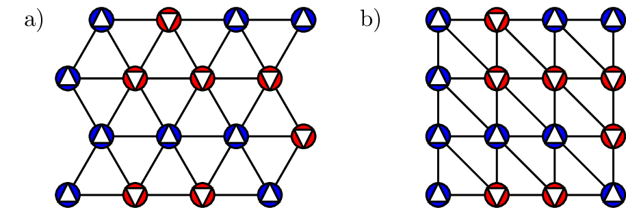
When implementing simulations the alternative view of the triangular lattice in Fig. 1b) can be useful for easier indexing of the lattice sites. For our purpose, we restrict ourselves to square dimensions of the lattice, i.e., \(N=L^2\) with edge length \(L\).

1.1.1 Geometric frustration

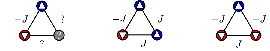
The phenomenon of geometric frustration arises on the triangular lattice in the case of antiferromagnetic interactions between the spins, i.e., \(J>0\). To get a first intuition for the low temperature behavior of the system, it is instructive to consider spin configurations on a single triangular plaquette that minimize the energy. Clearly, one can always minimize the energy contribution coming from two neighboring spins along one of the bonds, by aligning them antiparallel. However, the third spin can only be antiparallel to one of the two others as shown in Fig. 2, meaning that the minimal attainable energy is \(-J\) and six of the eight possible configurations have this energy. This phenomenon of competing interaction energies that cannot be simultaneously minimized due to the lattice geometry and thereby lead to degenerate minimal-energy configurations is called geometric frustration. When considering the full triangular lattice you will realize that the generalization of the previous considerations for an individual plaquette leads to a very large number of distinct microscopic states that minimize the energy, which is in stark contrast to an (anti-)ferromagnet on a square lattice, where fixing the orientation of one spin immediately determines the complete minimal energy configuration.

One central result of this lab course project will be that the number of minimal energy configurations in the triangular antiferromagnet is in fact so large that it exhibits a non-vanishing zero-point entropy. The system fluctuates within this large manifold of states, which effectively prohibits any ordering at low temperatures and there is no finite-temperature phase transition at all. This residual entropy was first calculated analytically by Wannier  [1,2], who obtained the value \(S_0/N=0.323\), where \(N\) is the number of lattice sites. Here you will explore thermodynamic signatures of this extensive residual entropy and learn how to accurately determine its value. Most strikingly, however, is the fact that the low-temperature physics associated with this residual entropy is associated with emergent magnetostatics – a concept which we discuss in more detail below. In addition, you will investigate the effect of applying an additional magnetic field, which alleviates the effects of the antiferromagnetic interactions, because it favors configurations where all magnets align with the magnetic field direction.

1.1.1.1 Emergent magnetostatics

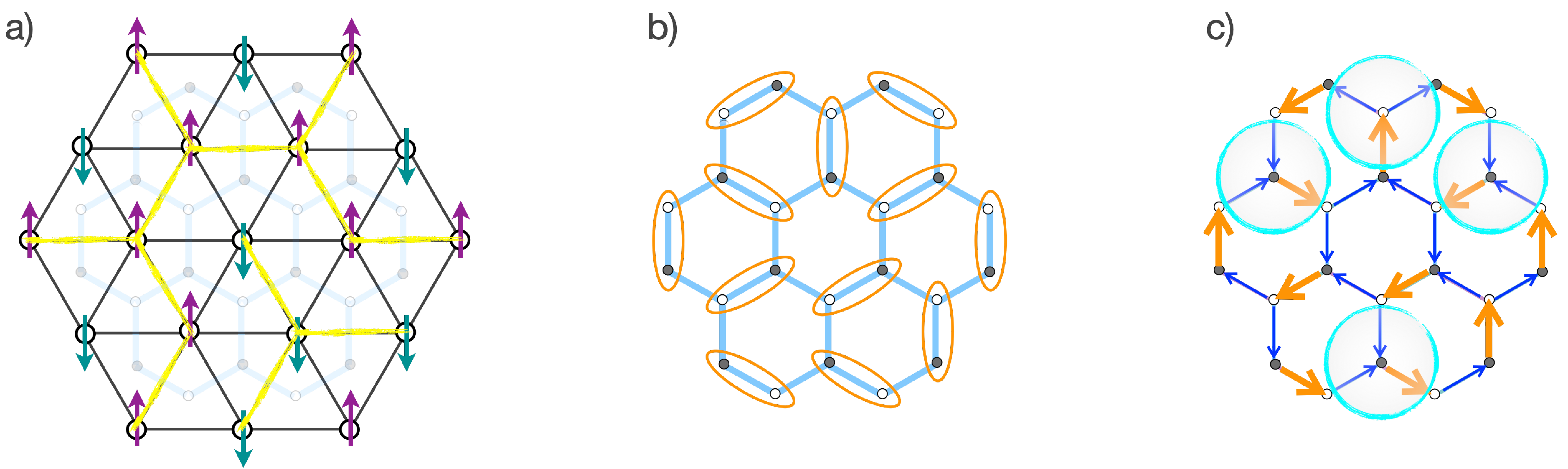
The low-temperature physics of the triangular Ising model with antiferromagnetic couplings is strikingly different from its ferromagnetic counterpart: While the ferromagnet exhibits a thermal phase transition at which the Z\(_2\) (Ising) symmetry of the Hamiltonian is spontaneously broken and the ground states exhibit less symmetry than the high-temperature paramagnetic phase, something much richer happens in the antiferromagnetic case – the ground states of the antiferromagnetic Ising model exhibit an emergent structure that is completely absent at high temperatures. This structure is called a Coulomb phase  [3] or emergent magnetostatics, in which every ground-state spin configuration can be mapped (as illustrated in Fig. 3) to an effectively divergence-free magnetic field configuration, hence the name magnetostatics.

Here is a short video introducing you to this idea, the exact mapping of a ground-state spin configuration to a divergence-free magnetic field configuration (see Fig. 3), and its ramifications in terms of long-range correlations:

1.2 Thermodynamics and Statistical Physics

Statistical physics provides the theoretical framework to describe the macroscopic properties of systems that are composed of many microscopic degrees of freedom, such as the frustrated magnet introduced in Section 1.1. Since we are interested in the behavior of the magnet as we vary temperature, the central object of interest is the canonical partition function \[\begin{aligned} Z_\beta = \sum_{\mathbf s}e^{-\beta H(\mathbf s)}\ , \end{aligned}\qquad{(2)}\] where \(\beta=1/k_BT\) denotes the inverse temperature and the sum runs over all possible configurations of the spins; for our purpose we choose to set \(k_B=1\) in the following. The individual terms that are summed are the Boltzmann weights that describe the contribution of the corresponding configuration to the canonical ensemble at the given temperature and, accordingly, \[\begin{aligned} p_\beta(\mathbf s)=\frac{1}{Z_\beta}e^{-\beta H(\mathbf s)} \end{aligned}\qquad{(3)}\] is the probability of encountering a specific configuration \(\mathbf s\) in the ensemble. The macroscopic quantities of interest are expectation values with respect to this Boltzmann distribution. The central role of the partition function is due to the fact that these expectation values can always be written as a derivative of the (logarithmic) partition function (potentially after introducing some auxiliary source terms). For example, the energy expectation value is \[\begin{aligned} \langle E\rangle_\beta =-\frac{\partial}{\partial\beta}\log Z_\beta =-\frac{\partial}{\partial\beta}\log\bigg(\sum_{\mathbf s}e^{-\beta H(\mathbf s)}\bigg) =\frac{1}{Z_\beta}\sum_{\mathbf s}H(\mathbf s)e^{-\beta H(\mathbf s)}\ , \end{aligned}\qquad{(4)}\] and, accordingly, the specific heat for some temperature \(T=1/\beta\) at constant volume is \[\begin{aligned} c_V(T) =\lim_{\Delta T\to0}\frac{\Delta Q}{\Delta T}=\frac{1}{V}\frac{\partial}{\partial T}\langle E\rangle_\beta=-\frac{1}{V}\frac{\partial}{\partial T}\frac{\partial}{\partial\beta}\log Z_\beta\ . \end{aligned}\qquad{(5)}\] In the latter expression \(\Delta Q\) denotes the head added to the system to raise its temperature by \(\Delta T\).

1.2.1 Entropy

For the purpose of this lab course experiment we will combine the two different viewpoints of entropy taken in thermodynamics and statistical physics, namely entropy being

1. a thermodynamic function of state, and

2. an information theoretic measure for the ignorance about the microscopic state.

1.2.1.1 Entropy in Statistical Physics

For a random variable \(X\) with probability distribution \(P(X)\) the Shannon entropy is defined as \[\begin{aligned} H(X) = -\sum_x P(X=x)\log_2 P(X=x)\ . \end{aligned}\qquad{(6)}\] The functional form of \(H\) is chosen such that it can be interpreted as a measure for the uncertainty about the outcome \(x\), because \(H\) is maximal for a uniform distribution and minimal for deterministic outcomes with \(P(X=x_0)=1\). In the form of Eq. 6 entropy is a central quantity in modern information theory, where it quantifies the information content of a message. Remarkably, Ludwig Boltzmann had already long before identified that a closely related quantity that builds on the microscopic states of a system and fulfils the properties of thermodynamic entropy, namely \[\begin{aligned} S=k_B\ln\Omega\ . \end{aligned}\qquad{(7)}\] Here, \(k_B\) is the Boltzmann constant and \(\Omega\) denotes the phase space volume accessible by the microscopic states given the known macroscopic variables. An equivalent expression is \[\begin{aligned} S = -k_B\sum_xp(x)\ln p(x)=\frac{k_B}{\ln 2}H(X) \ . \end{aligned}\qquad{(8)}\] In this case \(x\) denotes the microscopic states and \(p(x)\) is the probability of this state in the given statistical ensemble. This latter formulation reveals the direct relation to Shannon entropy.

1.2.1.2 Thermodynamic entropy

In thermodynamics, the entropy \(S\) was introduced by Rudolf Claudius as an extensive function of state. In a reversible process, where the added heat is \(\delta Q_{\text{rev}}\) at temperature \(T\), the differential of entropy is \[\begin{aligned} dS=\frac{\delta Q_{\text{rev}}}{T}\ . \end{aligned}\qquad{(9)}\] Since \(dS\) is a total differential, the entropy change in a reversible process is path independent. This reflects the fact that entropy is a function of state, because once the entropy is fixed for a value of the thermodynamic variables \(X_0\), it can be determined at any other point via \[\begin{aligned} S(X) = S(X_0)+\int_{X_0}^X\frac{\delta Q_{\text{rev}}}{T}\ . \end{aligned}\qquad{(10)}\]

1.2.2 Phase transitions

At a phase transition a small change of some control parameter (e.g., temperature or applied magnetic field) leads to a rapid qualitative change of the properties of the system. Formally, phase transitions are signaled by a non-analyticity of a thermodynamic potential, or, equivalently, zeros of the partition function 2.

The ferromagnetic Ising model on the triangular lattice exhibits such a thermal phase transition between a ferromagnetic and a paramagnetic phase at the critical temperature \(T_c=3.6403\)  [4]. At this continuous phase transition the specific heat 5, which is the second derivative of the free energy, diverges as a power law, \[\begin{aligned} c_V(T)\sim|T-T_c|^{-\alpha}\ . \end{aligned}\qquad{(11)}\]

1.3 Monte Carlo simulation

A central challenge in statistical physics is due to the fact that it is in most cases not possible to handle the partition sum 2 analytically and the numerical cost of naively computing it quickly explodes because of the combinatorially large number of microscopic configurations that has to be summed over. Hence, it is in practice typically impossible to work with the normalized Boltzmann weights \(p_\beta(\mathbf s)\). In this lab course project you will use a numerical approach that circumvents the issue of computing the partition sum by resorting to a Monte Carlo sampling algorithm for which knowing the unnormalized Boltzmann weights \[\begin{aligned} \tilde p_\beta(\mathbf s) = e^{-\beta H(\mathbf s)} \end{aligned}\qquad{(12)}\] is sufficient  [5]. But most importantly, Monte Carlo sampling will also allow you to avoid traversing the exponentially large configuration space, but ingeniously allow you to converge expectation values of physical observables in polynomial time.

1.3.1 Monte Carlo estimation of expectation values

In statistical physics we are usually interested in expectation values of the form \[\begin{aligned} \langle{O}\rangle_\beta=\sum_{\mathbf s}p_\beta(\mathbf s)O(\mathbf s)\ , \end{aligned}\qquad{(13)}\] where \(O(\mathbf s)\) is some function of the microscopic configuration \(\mathbf s\), such as some observable like energy, magnetization, or two-point correlation functions. Assume that we have a means to obtain a finite sample \(\mathcal S_M=\{\mathbf s_1,\ldots,\mathbf s_M\}\) such that in the limit of large \(N\) the relative frequency of a configuration \(\mathbf s\) in \(\mathcal S_M\) is proportional to its probability \(p_\beta(\mathbf s)\). Then, according to the law of large numbers, the sample mean converges to the expectation value with increasing sample size, \[\begin{aligned} \langle\langle O\rangle\rangle_N\equiv\frac{1}{N}\sum_{\mathbf s\in\mathcal S_M}O(\mathbf s)\overset{M\to\infty}{\longrightarrow}\langle{O}\rangle_\beta\ . \end{aligned}\qquad{(14)}\] Moreover, given the variance \(\sigma_O^2=\sum_{\mathbf s}p_\beta(\mathbf s)(O(\mathbf s)-\langle{O}\rangle_\beta)^2\) the expected deviation of the sample mean from the exact expectation value is \[\begin{aligned} \Delta_O^M=\sqrt{\mathbb E\big((\langle\langle O\rangle\rangle_M-\langle{O}\rangle_\beta)^2\big)}=\frac{\sigma_O}{\sqrt{M}}\ , \end{aligned}\qquad{(15)}\] if the \(\mathbf s_j\) are independent samples. This means that, given a finite sample \(\mathcal S_M\), we can obtain an estimate of the expectation value together with a corresponding error estimate as \[\begin{aligned} \langle{O}\rangle_\beta=\langle\langle O\rangle\rangle_M\pm\frac{\sigma_O}{\sqrt{M}}\ . \end{aligned}\qquad{(16)}\]

1.3.2 Metropolis-Hastings algorithm

The idea of the Metropolis-Hastings algorithm is to realize a Markov process whose stationary distribution is the probability distribution \(\pi(\mathbf s)\) that we are interested in. Once the process reached its stationary state, the states \(\mathbf s_i\) visited can be used as a sample \(\mathcal S_M\) and therefore to estimate expectation values.

In a Markov process the system is described by a state \(\mathbf s\) and in each time step it transitions into a new state \(\mathbf s'\) according to a transition probability \(p_{MC}(\mathbf s\to\mathbf s')\equiv p_{MC}(\mathbf s'|\mathbf s)\) that only depends on the current state of the system, i.e. there is no memory of the past trajectory. In the Metropolis-Hastings algorithm the Markov transition probabilities are constructed in two steps, given the current state \(\mathbf s\). First, a new configuration \(\mathbf s'\) is proposed following a proposal probability \(p_P(\mathbf s'|\mathbf s)\) that can be conditioned on the current state. Given the proposed configuration \(\mathbf s'\) the update is accepted with a probability \[\begin{aligned} p_A(\mathbf s,\mathbf s')=\text{min}\bigg(1,\frac{\pi(\mathbf s')}{\pi(\mathbf s)}\frac{p_P(\mathbf s|\mathbf s')}{p_P(\mathbf s'|\mathbf s)}\bigg) \ . \end{aligned}\qquad{(17)}\] Hence, the probability to move from state \(\mathbf s\) to state \(\mathbf s'\) in the resulting Markov process is \[\begin{aligned} p_{MC}(\mathbf s\to\mathbf s')=p_P(\mathbf s'|\mathbf s)p_A(\mathbf s,\mathbf s')\ . \end{aligned}\qquad{(18)}\] This form of the transition probability is chosen to satisfy the detailed balance condition \[\begin{aligned} \pi(\mathbf s)p_{MC}(\mathbf s\to\mathbf s')=\pi(\mathbf s')p_{MC}(\mathbf s'\to\mathbf s)\ , \end{aligned}\qquad{(19)}\] which is a sufficient condition for the Markov process to have \(\pi(\mathbf s)\) as stationary distribution. Uniqueness of the stationary distribution is guaranteed if the process is ergodic, i.e., if it is possible for the process to go from any state \(\mathbf s\) to any other state \(\mathbf s'\) in a finite number of steps. Clearly, the latter condition has to be kept in mind when designing the proposal probability \(p_P(\mathbf s'|\mathbf s)\).

For Ising spin systems single spin flip updates are often sufficient. This means that from the given configuration \(\mathbf s\) one flips the sign of a single degree of freedom, \(s_i'=-s_i\), and the proposal probability \(p_P(\mathbf s'|\mathbf s)\) is a uniform distribution over all configurations \(\mathbf s'\) that differ from \(\mathbf s\) by a single spin flip. To reduce the cost of estimating expectation values and to mitigate the effect of autocorrelation discussed in the following section, one typically performs sweeps of local updates between subsequent configurations that are added to the sample \(\mathcal S_M^{\text{MC}}\). One sweep consists of one Markov update step per degree of freedom, which means that the configuration obtained after the update sweep can globally differ from the initial configuration.

1.3.3 Thermalization and Autocorrelation

For an infinite Markov chain \(\mathcal S_{\infty}^{MC}=\{\mathbf s_1,\mathbf s_2,\ldots\}\) constructed using the Metropolis-Hastings algorithm the frequency of configuration \(\mathbf s\) is proportional to its probability \(\pi(\mathbf s)\). However, when working with finite samples \(\mathcal S_{M}^{MC}\), some additional care is required. Fig. 4a shows the value of some observable \(O(\mathbf s)\) evaluated on a sequence of configurations \(\mathbf s\) that were obtained using the Metropolis-Hastings algorithm. The data exhibits two typical features of Markov chain Monte Carlo, namely an initial thermalization period and a significant autocorrelation time. By contrast, the trajectory shown in Fig. 4b evolves around a stationary value and signatures of autocorrelation are much less pronounced.

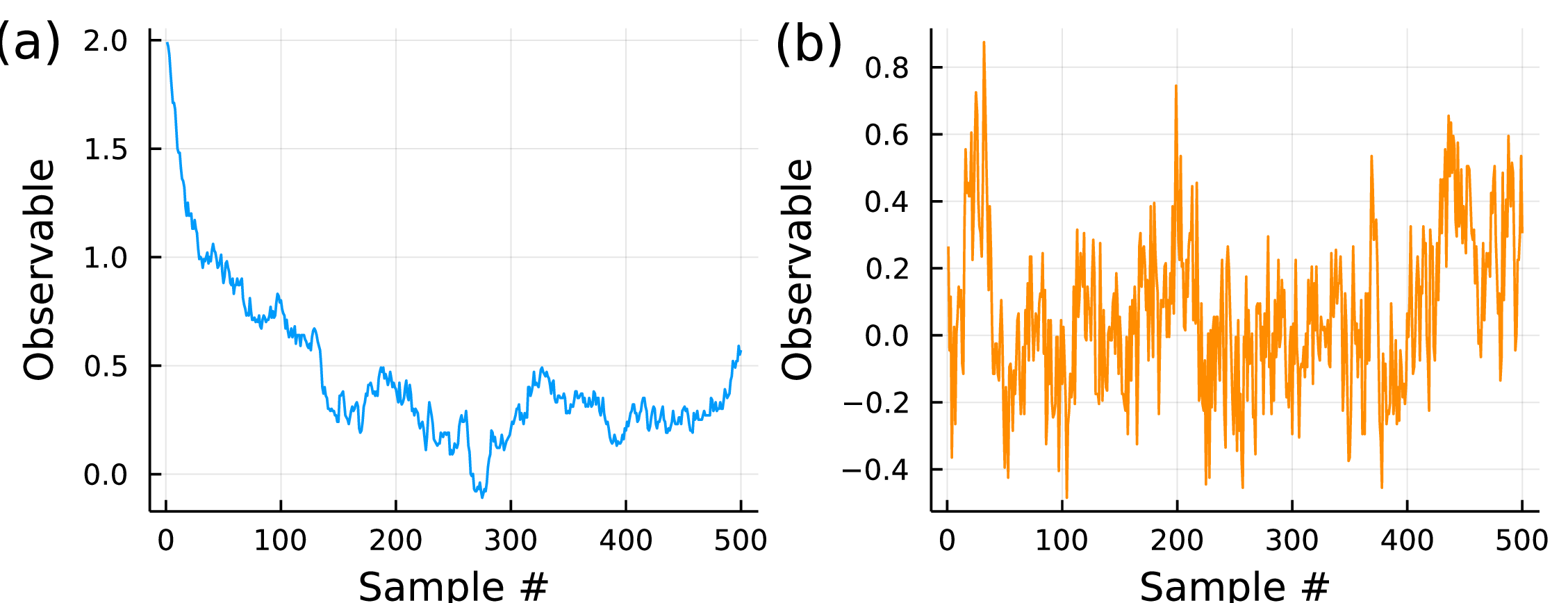
Thermalization (or burn in) refers to the initial part of the trajectory, during which the process approaches the stationary state. The first configuration \(\mathbf s_1\) is usually chosen to be either random or completely ordered and it is usually not a typical state of the target distribution \(\pi(\mathbf s)\). Therefore, it takes a number of steps for the Markov process to thermalize, i.e., to reach states that are typical, and, thereby, the stationary region. In practice, the configurations sampled during the thermalization period have to be discarded, because they would otherwise introduce an unintended bias to the sample \(\mathcal S^{MC}_M\). Determining the duration of the initial thermalization period is usually one of the first steps when performing a Markov chain Monte Carlo simulation.

The signature of autocorrelation in Fig. 4a is the fact that one can throughout the stationary part of the trajectory still identify clear periods of upwards or downwards trends. This means that consecutive samples in the sequence are correlated with each other. This behavior is a problem when we estimate expectation values according to Eq. 16, because the error estimation based on the standard deviation assumes independently drawn samples. Clearly, correlated samples are not independent and therefore, the error as given in Eq. 15 would underestimate the actual deviation.

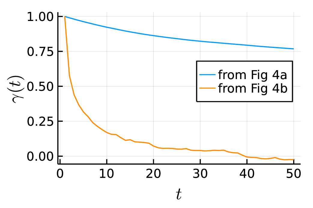
Considering the sequence of configurations \(\mathbf s_1,\ldots,\mathbf s_M\), the autocorrelation is quantified by the correlation function \[\begin{aligned} \gamma(t)=\frac{\mathbb E\big[O(\mathbf s_n)O(\mathbf s_{n+t})\big]-\mathbb E\big[O(\mathbf s)\big]^2}{\text{Var}\big[O(\mathbf s)\big]} \end{aligned}\qquad{(20)}\] where the expectation values \(\mathbb E[\cdot]\) and the variance \(\text{Var}\big[\cdot\big]\) are in practice estimated via the sample mean over the given sequence. Fig. 5 shows the autocorrelation function for the data shown in Fig. 4. It exhibits that correlations between samples in Fig. 4a remain significant for more than fifty steps of the Monte Carlo chain, while it rapidly drops in the case of Fig. 4b, meaning that subsequent samples are almost uncorrelated. The characteristic number of steps required for the decay of the autocorrelation is called the autocorrelation time \(\tau\).

If the autocorrelation time of the data is known, it can be used to correct the error estimate of Eq. 15 by defining an effective number of uncorrelated samples, \(M_{\text{eff}}=M/(1+2\tau)\)  [6]. With this, the error estimate becomes \[\begin{aligned} \Delta_O^M=\frac{\sigma_O}{\sqrt{M_{\text{eff}}}}=\frac{\sigma_O}{\sqrt{M}}\sqrt{1+2\tau}\ . \end{aligned}\qquad{(21)}\]

For this purpose, it is required to estimate the autocorrelation time. One option is to assume an exponential form of the autocorrelation function, \(\gamma(t)\propto e^{-t/\tau}\), and to extract \(\tau\) by fitting to the data or by computing the integrated autocorrelation time \(\tau = \sum_{t=1}^{\infty}\gamma(t)\). However, this is often not practical. A viable alternative is to extract the autocorrelation time from a binning analysis of the data. This approach is explained as part of the general purpose toolbox on the lab course website  [7].

2 Preparation

2.1 Theory

While you familiarize yourself with the theoretical background, find answers to the following questions. You will need those for the analysis of the Monte Carlo data.

1. Considering the definition of the specific heat \(c_V\) in Eq. 5, what quantity that is a function of the microscopic configurations \(\mathbf s\) can you use to compute \(c_V\) in a Monte Carlo simulation?

2. What is the entropy of the frustrated magnet at infinite temperature (\(\beta=0\))?

3. Assuming that you know the specific heat as a function of temperature, \(c_V(T)\), how can you use Eq. 10 and your answer to [q1] to determine the entropy at \(T=0\)?

4. Convince yourself that the Metropolis-Hastings acceptance probability 17 fulfills the detailed balance condition 19.

2.2 Coding

In this lab course project you will write your own implementation of a Markov chain Monte Carlo simulation for the triangular lattice Ising model. You likely implemented such a simulation for another Ising model before. In that case you might use your existing code as a basis for this project.
When composing the simulation from scratch, the central building blocks that you need to implement are the following:

1. Write a function that computes the total energy \(H_{J,B}(\mathbf s)\) according to Eq. 1 for a given spin configurations \(\mathbf s\) and given parameters \(J\) and \(B\).

2. For a performant implementation it is useful to have a function that computes the energy difference of configurations \(\mathbf s\) and \(\mathbf s'\) that differ by a single flipped spin \(s_i'=-s_i\), \[\begin{aligned} \Delta E_{J,B}(\mathbf s; i)=H_{J,B}(\mathbf s')-H_{J,B}(\mathbf s)=-2s_i\sum_{j\in\mathcal N_i}s_j\ . \end{aligned}\qquad{(22)}\] Here, \(\mathcal N_i\) denotes the neighboring lattice sites of site \(i\). This function is useful to compute acceptance probabilities for single spin flip updates. Cross-check your function for the total energy and your function for the energy differences to ensure a correct implementation.

3. Write a function that performs an update sweep starting from a given configuration \(\mathbf s\) and that returns the updated configuration \(\mathbf s'\). The sweep should consist of \(N\) Markov steps.
   

\begin{algorithm}
\caption{Pseudocode for update sweep function}
\begin{algorithmic}
\Function{sweep}{$\vec s$, $T$}
\For{$n$ in $1:N$}
\State $i\leftarrow$random\_int(1,N)
\State $\Delta E\leftarrow\Delta E_{J,B}(\vec s, i)$
\State $p_{\text{acc}}=\exp(-\Delta E/T)$
\If{random\_float(0,1) $< p_{\text{acc}}$} 
\State $\vec s\leftarrow$flip($\vec s,i$)
\EndIf
\EndFor
\State
\Return $\vec s$
\EndFunction
\end{algorithmic}
\end{algorithm}

4. Write a function that generates a sample \(\mathcal S_M^{MC}\) of given size \(M\) by running the Markov chain and storing the current configuration \(\mathbf s\) between successive update sweeps.

5. Write a function that performs a binning analysis for a given sequence of observables \(O_i=O(\mathbf s^{(i)})\) following the instructions given on the toolbox page  [7]

3 Tasks

3.1 Ferromagnet \(J<0\)

For this part, we fix \(B=0\) and we consider a range of linear system sizes \(L=10,20,40,80\).

1. Determine a suited grid for the temperature axis. For this purpose, generate samples of size \(M=2\times10^4\) for system size \(L=20\) at different temperatures \(1\leq T/|J|\leq6\). Compute the expectation value of the squared magnetization \(M^2(\mathbf s)=\big(\frac{1}{L^2}\sum_j s_j\big)^2\) to identify in which regions you need higher resolution in temperature.

2. For \(L=40\): Compute and plot the autocorrelation function \(\gamma(t)\) defined in Eq. 20 for three temperatures, below, close to, and above the critical temperature, using the energy and the squared magnetization \(M^2\) as the observables. What do you observe?

3. For \(L=10,20\), convince yourself that the sequence of error estimates of the binning analysis converges as function of the coarse-graining size \(k\). Determine the autocorrelation time \(\tau\) at each temperature. How does the autocorrelation time depend on system size and temperature?

4. Compute the expectation values of the squared magnetization \[\begin{aligned} M^2(\mathbf s)=\Big(\frac{1}{L^2}\sum_j s_j\Big)^2\ . \end{aligned}\qquad{(23)}\] What do you observe as temperature and system size are varied?

5. Compute the specific heat for all system sizes as function of temperature. What do you observe as temperature and system size are varied?

3.2 Antiferromagnet \(J>0\)

Choose a temperature grid that is evenly spaced on a logarithmic scale, e.g., \(T_n/J=2^{n/4}\) for \(n=-12,\ldots,28\) and generate Monte Carlo samples for these temperatures with linear system sizes \(L=10,20,40,80\).

6. For your samples for \(L=10,20\), convince yourself that the sequence of error estimates of the binning analysis converges as function of the coarse-graining size \(k\). Determine the autocorrelation time \(\tau\) at each temperature. How does the autocorrelation time depend on system size and temperature?

7. Compute the specific heat as function of temperature for each system size. Compare the behavior to your results for the ferromagnet.

8. Using the specific heat obtained in 7, compute the zero-point entropy of the frustrated magnet. How does the value you find compare with the exact value from the literature? Discuss possible deviations.

9. For \(L=40\), at a fixed small temperature (e.g. \(T/J=0.2\)), generate samples for a grid of magnetic field values \(B\in[0,10]\). Compute the magnetization as a function of the magnetic field. What do you observe? How can you explain your observation?

10. (optional) For \(L=80\), calculate the spin-spin correlation function \(\langle s_0 s_i \rangle\) along a (horizontal) cut in the lattice, where \(s_0\) is a selected spin along this cut and \(s_i\) are the remaining 79 spins along the cut. Investigate the decay of this spin-spin correlation function for high and low temperatures (e.g. \(T/J=1.0\) and \(T/J=0.1\)) as a function of real-space distance. You can also compare this to the ordered phase of the ferromagnetic model.

References

Materials

• Instruction PDF
• Toolbox: Binning analysis