Tensor networks

1 Theory

1.1 Introduction

A central feature of physical systems that are composed of many interacting degrees of freedom are phase transitions. At a phase transition the collective behavior of the system exhibits an abrupt qualitative change as some external control parameter is varied. A paradigmatic example is the continuous transition of the two-dimensional Ising magnet between a ferromagnetic phase at low temperatures and a paramagnetic phase at high temperatures. This simple model allows us to understand that thermal fluctuations eventually destroy the macroscopic magnetization of the system as the temperature is increased; in that sense, we say that this phase transition is driven by thermal fluctuations.

Remarkably, phase transitions can also occur at zero temperature – so-called quantum phase transitions. The crossing of a quantum phase transition means that the ground state properties of a quantum many-body system suddenly change qualitatively as some external control parameter is tuned. In this case, the transition is driven by quantum fluctuations instead of thermal fluctuations. In this project you will investigate numerically two examples of quantum phase transitions.

Addressing quantum many-body systems numerically, however, poses a formidable challenge. Since the many-body Hilbert space is constructed as the tensor product of the single particle Hilbert spaces, the Hilbert space dimension grows exponentially with the number of degrees of freedom. In naive approaches this translates into exponential amounts of computational resources required to simulate quantum many-body systems. Interestingly, however, the low-energy regime exhibits additional structure in the wave functions, which can be exploited for compressed representations. In this project, you will work with tensor network wave functions that are ideally suited to encode the ground states of low-dimensional quantum systems.

1.2 Quantum phase transitions

Just as thermal phase transitions, quantum phase transitions feature fluctuations that encompass all length and time scales  [1]. As the transition point is approached, the correlation length diverges as \[\begin{aligned} \xi\propto|\epsilon|^{-\nu}\ , \end{aligned}\qquad{(1)}\] where \(\epsilon\) denotes a dimensionless measure of the distance to the critical point and \(\nu\) is the correlation length critical exponent.¹ Simultaneously, the correlation time diverges as \[\begin{aligned} \tau_c\propto \xi^z\propto|\epsilon|^{-z\nu} \end{aligned}\qquad{(2)}\] with the dynamical critical exponent \(z\). Close to the critical point, \(\xi\) and \(\tau_c\) are the unique characteristic length and time scales. Therefore, the dependence of any observable on external parameters is determined by their relation to the diverging characteristic scales. For example, an observable \(O(x,t)\), that depends on space and time as external parameters, can be written in terms of a scaling function \(F_O\) as \[\begin{aligned} O(x,t)=F_O(x/\xi,t/\tau_c) \end{aligned}\qquad{(3)}\] This is the core of so-called critical behavior close to a phase transition, which is fully characterized by the critical exponents. For the purpose of this project we restrict the discussion to finite size scaling of dimensionless quantities; in other cases, an appropriate dimensionful prefactor has to be added to the scaling function above.

In practice with numerical simulations, however, one often introduces an additional length scale, namely, the system size \(L\). This typically has a significant impact close to the phase transition. Imagine, for example a quantity \[\begin{aligned} A(\epsilon)\propto|\epsilon|^\zeta\propto\xi^{\zeta/\nu} \end{aligned}\qquad{(4)}\] that diverges with some exponent \(\zeta\) at the critical point. In a finite system the correlation length is bounded by \(L\), such that we obtain the finite size behavior \[\begin{aligned} A_L(\epsilon)\propto L^{\zeta/\nu} \end{aligned}\qquad{(5)}\] close to the transition. This means, that close to the critical point, some quantities of interest can exhibit strong (seemingly divergent) dependence on the system size and need to be treated with care. On the other hand, the system size \(L\) thereby becomes a control parameter and suited finite size scaling can allow us to determine the value of critical exponents.

 

In quantum systems a characteristic feature of the energy spectrum that is related to the characteristic time scale is the energy gap between the ground state and the first excited state, \(\Delta E\). From dimensional considerations we obtain \[\begin{aligned} \Delta E\propto \tau_c^{-1}\propto\xi^{-z}\propto|\epsilon|^{z\nu}\ . \end{aligned}\qquad{(6)}\] This means that the divergence of the correlation time scale at the critical point corresponds to a closing of the energy gap, which is characteristic for quantum phase transitions. In the presence of a finite size cutoff one can extend this behavior to a scaling ansatz for the gap in the vicinity of the phase transition point, \[\begin{aligned} \Delta E_L(\epsilon)=L^{-z}F_{\Delta E}(\epsilon/L^{-1/\nu})\ . \end{aligned}\qquad{(7)}\] Given numerical data such finite size scaling forms can be probed by attempting a so-called scaling collapse. This means for this example that the numerical data points \(\Delta E_L(\epsilon)\) for different system sizes \(L\) and different values of \(\epsilon\) are plotted on rescaled axes such that all data points lie on a line given by \(y=F_{\Delta E}(x)\). Concretely, this means that \(y=L^z\Delta E_L\) and \(x=\epsilon/L^{-1/\nu}\).

As part of this project you will probe such finite size scaling relations numerically.

1.3 Model Hamiltonians

In this project we will be concerned with to model systems that exhibit interesting quantum phases of matter, namely the transverse-field Ising model and the bilinear-biquadratic spin-1 chain. The former is the drosophila of quantum phase transitions and the latter admits an exact tensor network representation of the ground state as well as interesting phenomena like fractionalization.

1.3.1 Transverse-field Ising model

The transverse-field Ising model is the paradigmatic model for a quantum phase transition. It incorporates the energetic competition between a ferromagnetic coupling term of neighboring spin-1/2 degrees of freedom and an external magnetic field \(g\) that is oriented along the transverse direction, \[\begin{aligned} \hat H_{\text{TFIM}}=-\sum_{i=1}^{L-1}\hat S_i^z\hat S_{i+1}^z-g\sum_{i=1}^L\hat S_i^x\ . \end{aligned}\qquad{(8)}\] Acting on the local spin-1/2 Hilbert spaces, the spin operators have the matrix representation \[\begin{aligned} \hat S^x=\frac12\begin{pmatrix}0&1\\1&0\end{pmatrix} \quad\text{and}\quad \hat S^z=\frac12\begin{pmatrix}1&0\\0&-1\end{pmatrix} \end{aligned}\qquad{(9)}\] At \(g=0\) the system exhibits a degenerate manifold of ferromagnetically ordered ground states spanned by \[\begin{aligned} |{\psi_0^{(+)}}\rangle=|{\uparrow,\ldots,\uparrow}\rangle+|{\downarrow,\ldots,\downarrow}\rangle \end{aligned}\qquad{(10)}\] and \[\begin{aligned} |{\psi_0^{(-)}}\rangle=|{\uparrow,\ldots,\uparrow}\rangle-|{\downarrow,\ldots,\downarrow}\rangle\ . \end{aligned}\qquad{(11)}\] At \(g=\infty\) the unique ground state is the transversely polarized product state \[\begin{aligned} |{\psi_0}\rangle=|{\rightarrow,\ldots,\rightarrow}\rangle=\frac{1}{2^{L/2}}\bigotimes_{i=1}^L\big(|{\uparrow}\rangle_i+|{\downarrow}\rangle_i\big)\ . \end{aligned}\qquad{(12)}\] In the thermodynamic limit \(L\to\infty\), the system undergoes a symmetry-breaking phase transition at some intermediate \(0<g_c<\infty\). The corresponding order parameter is the longitudinal magnetization \[\begin{aligned} \hat M_z=\frac{1}{L}\sum_{i=1}^L\hat S_i^z\ . \end{aligned}\qquad{(13)}\] As symmetry-breaking will, however, only occur in the thermodynamic limit, the ground state expectation value \(\langle{\hat M_z}\rangle\) will always be zero in numerical studies of finite systems. Instead, one can resort to the squared magnetization \(\hat M_z^2\) as an indicator of ordering in finite systems.

1.3.2 Bilinear-biquadratic spin-1 chain

The Hamiltonian of the bilinear-biquadratic spin-1 chain is defined as \[\begin{aligned} \hat H_{\text{BLBQ}}=\cos\theta\sum_{i=1}^{L-1}\hat{\mathbf S}_i\cdot\hat{\mathbf S}_{i+1}+\sin\theta\sum_{i=1}^{L-1}\big(\hat{\mathbf S}_i\cdot\hat{\mathbf S}_{i+1}\big)^2 \end{aligned}\qquad{(14)}\] Here, we use the notation \[\begin{aligned} \hat{\mathbf S}_i\cdot\hat{\mathbf S}_{i+1} = \hat S_i^x\hat S_{i+1}^x+\hat S_i^y\hat S_{i+1}^y+\hat S_i^z\hat S_{i+1}^z = \frac12\big(\hat S_i^+\hat S_{i+1}^-+\hat S_i^-\hat S_{i+1}^+\big)+\hat S_i^z\hat S_{i+1}^z \end{aligned}\qquad{(15)}\] and the spin-1 operators have the matrix representation \[\begin{aligned} \hat S^x=\frac{1}{\sqrt 2}\begin{pmatrix}0&1&0\\1&0&1\\0&1&0\end{pmatrix} \ \text{,}\quad \hat S^y=\frac{1}{\sqrt 2i}\begin{pmatrix}0&1&0\\-1&0&1\\0&-1&0\end{pmatrix} \quad\text{and}\quad \hat S^z=\begin{pmatrix}1&0&0\\0&0&0\\0&0&-1\end{pmatrix}\ . \end{aligned}\qquad{(16)}\] As the parameter \(\theta\) is varied, the bilinear-biquadratic spin-1 model exhibits a rich phase diagram. One point of particular interest is \(\tan\theta=\frac13\), the Affleck-Kennedy-Lieb-Tasaki (AKLT) point. It has been shown by AKLT that the ground state at this point can be constructed as depicted in Fig. 1. In this construction the local spin-1 Hilbert space is viewed as the triplet subspace of two fictitous spin-1/2 degrees of freedom, i.e., \[\begin{aligned} |{+}\rangle=|{\uparrow\uparrow}\rangle\ ,\quad |{0}\rangle=\frac{|{\uparrow\downarrow}\rangle+|{\downarrow\uparrow}\rangle}{\sqrt2}\ ,\quad |{-}\rangle=|{\downarrow\downarrow}\rangle\ . \end{aligned}\qquad{(17)}\] The AKLT ground state is then obtained by pairing the spin-1/2 states on neighboring sites in to singlets and subsequently projecting onto the triplet subspace of each site.

Remarkably, this prescription immediately translates into a tractable matrix product form of the AKLT state. Let us denote by \(a_i=\uparrow,\downarrow\) and \(b_i=\uparrow,\downarrow\) the local quantum numbers of the two auxiliary spin-1/2 degrees of freedom at lattice site \(i\). Then \(|{\mathbf a,\mathbf b}\rangle\) denotes a basis state of the auxiliary spin-1/2 system. As mentioned above, the starting point is a product of singlets, which can be written as \[\begin{aligned} |{\tilde\psi_{a_1b_L}}\rangle=\sum_{a_2,\ldots,a_L}\sum_{b_1,\ldots,b_{L-1}}\Sigma_{b_1a_2}\Sigma_{b_2a_3}\ldots\Sigma_{b_{L-1}a_L}|{\mathbf a\mathbf b}\rangle \end{aligned}\qquad{(18)}\] with matrices \[\begin{aligned} \Sigma=\begin{pmatrix}0&\frac{1}{\sqrt2}\\-\frac{1}{\sqrt2}&0\end{pmatrix}\ . \end{aligned}\qquad{(19)}\] The indices of \(|{\tilde\psi_{a_1b_L}}\rangle\) indicate that the state of the first and the last spin-1/2 can be chosen arbitrarily due to the open boundary condition. Next, we perform the local projections with projection operators \[\begin{aligned} \hat P=\sum_{s=-,0,+}\sum_{a,b=\uparrow,\downarrow}P_{ab}^s|{s}\rangle\langle{ab}| \end{aligned}\qquad{(20)}\] defined by the tensors \[\begin{aligned} P^+=\begin{pmatrix}1&0\\0&0\end{pmatrix}\ ,\quad P^0=\begin{pmatrix}0&\frac{1}{\sqrt2}\\\frac{1}{\sqrt2}&0\end{pmatrix}\ ,\quad P^-=\begin{pmatrix}0&0\\0&1\end{pmatrix}\ . \end{aligned}\qquad{(21)}\] Thereby, we obtain \[\begin{aligned} |{\psi_{\text{AKLT}}^{ab}}\rangle&=\bigotimes_i\hat P_i|{\tilde\psi_{ab}}\rangle \nonumber\\ &= \sum_{\mathbf s}\sum_{a_2,\ldots,a_L} \sum_{b_1,\ldots,b_{L-1}} P^{s_1}_{a,b_1}\Sigma_{b_1a_2}\ldots P^{s_{L-1}}_{a_{L-1},b_{L-1}}\Sigma_{b_{L-1}a_L}P^{s_L}_{a_L,b}|{\mathbf s}\rangle \nonumber\\ &\equiv \sum_{\mathbf s}\sum_{a_2,\ldots,a_L} A^{s_1}_{aa_2}A^{s_2}_{a_2,a_3}\ldots A^{s_{L-1}}_{a_{s_{L-1}}a_{s_{L}}}P^{s_L}_{a_L,b}|{\mathbf s}\rangle\ . \end{aligned}\qquad{(22)}\] The simplified matrix product form in the last line is obtained by defining \[\begin{aligned} A_{a_{i}a_{i+1}}^{s_i}=\sum_{b}P^{s_i}_{a_i,b}\Sigma_{ba_{i+1}}\ . \end{aligned}\qquad{(23)}\] The four possible choices \((a,b)\in\{(\uparrow,\uparrow),(\downarrow,\uparrow),(\uparrow,\downarrow),(\downarrow,\downarrow)\}\) reflect a fourfold degeneracy of the AKLT groundstate in the case of open boundary conditions. The state is of special interest, because it exhibits a “hidden” order that is indicated by a non-vanishing expectation value of the string correlators \[\begin{aligned} \mathcal C^{\text{string}}_{i,j}=\langle{\psi|\hat S_i^ze^{i\pi\sum_{i<k<j}\hat S_k^z}\hat S_j^z|\psi}\rangle \end{aligned}\qquad{(24)}\] at arbitrary distances \(|i-j|\). In the AKLT state the value is exactly known, namely \[\begin{aligned} \mathcal C^{\text{string}}_{i,j}=-\frac{4}{9}\quad\text{for }|i-j|>2\ . \end{aligned}\qquad{(25)}\] By contrast, all two-point correlation functions decay exponentially, meaning that there is no local order parameter. One characteristic feature of this symmetry-protected topological order is the existence of localized edge states at the boundary of the system – the free spin-1/2 degrees of freedom of the AKLT state.

The abovementioned physical features are robust to tuning the parameter \(\theta\) away from the AKLT point. The explicit construction of the wave function as a product of small matrices works only at the AKLT point. However, highly accurate approximations of the ground state in the form of products of small matrices can be found numerically across the phase diagram. And, most remarkably, this generalizes to arbitrary one-dimensional quantum systems that exhibit a gap between the ground state and the first excited state. In the next section we will discuss how a general matrix product form of the wave function as in Eq. 22 can be used as the foundation of a family of versatile and controlled numerical algorithms.

1.4 Tensor networks

Tensor network techniques are applicable to composite quantum systems, where the total Hilbert space is constructed as the tensor product of the Hilbert spaces of the individual degrees of freedom, \[\begin{aligned} \mathcal H=\bigotimes_{l=1}^L\mathcal H_l\ . \end{aligned}\qquad{(26)}\] Accordingly, the wave function can be expanded in a computational basis as \[\begin{aligned} |{\psi}\rangle=\sum_{s_1,\ldots,s_L}c_{s_1,\ldots,s_L}|{s_1}\rangle\otimes\ldots\otimes|{s_L}\rangle\equiv \sum_{s_1,\ldots,s_L}c_{s_1,\ldots,s_L}|{s_1,\ldots,s_L}\rangle\ , \end{aligned}\qquad{(27)}\] where the \(s_l\) denote quantum numbers associated with the basis states \(|{s_l}\rangle\in\mathcal H_l\).

We will in the following consider cases, where the local Hilbert space dimension of all constituent degrees of freedom is identical, \(\text{dim}(\mathcal H_l)=d\). Hence, the total Hilbert space dimension is \(\text{dim}(\mathcal H)=d^L\). Tensor networks achieve a dimensional reduction of the quantum many-body problem by rewriting the wave function coefficients \(c_{s_1,\ldots,s_L}\) as a contraction of tensors. Thereby, the generally exponential dependence of the number of required parameters on the system size can be reduced to a polynomial dependence, if the physical structure of the state allows for such compression. For one-dimensional systems the simplest tensor network structure is that of matrix product states (MPS), which you will use throughout this project.

The explanations below follow in many parts closely the presentation in Ref.  [2].

1.4.1 Matrix product states

If you are completely new to the idea of tensor networks, you may also consider this video from the Computation Many-Body Physics lecture, in addition to the following explanation:

The idea of MPS is to compress the many-body wave function by decomposing the wave function coefficients into a product of matrices, \[\begin{aligned} c_{s_1,\ldots,s_L}=\sum_{a_1,\ldots,a_{L-1}}A^{s_1}_{a_1}A^{s_2}_{a_1a_2}\ldots A^{s_L}_{a_{L-1}}\ . \end{aligned}\qquad{(28)}\] To estimate the number of parameters used in the matrix product representation, we can assume that \(a_l=1,\ldots,\chi\) independent of \(l\). In that case, the MPS consists of \(\mathcal O(Ld\chi^2)\) parameters, which is a substantial reduction compared to the \(2^d\) wave function coefficients if the bond dimension \(\chi\) can be chosen to be small. In Section 1.4.3 we will see that there is a distinguished physical resource that determines whether the wave function can be represented faithfully with a small bond dimension \(\chi\) – the entanglement of bipartitions. But before that, we discuss a useful graphical notation in the context of tensor networks and how a MPS form of a given wave function can be obtained in a constructive way by using singular value decompositions.

1.4.1.1 Graphical notation.

To avoid clumsy formulas with abundant summations and indices as in Eq. 28, we introduce a graphical representation of tensors and tensor contractions called Penrose graphical notation. Generally, any tensor will be represented as a node that has one leg for each of its indices. For example, the wave function coefficient is a tensor with \(L\) legs:

A tensor contraction is indicated in this diagrammatic representation by joining the legs of two tensors corresponding to the index that is contracted. For example, the contraction of the first two tensors on the right hand side of Eq. 28 is represented as

With these conventions, we can rewrite Eq. 28 graphically as

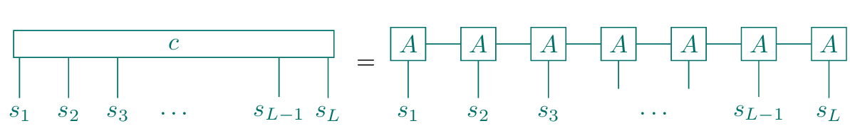
This pictorial representation of the MPS is the motivation to call the indices \(a_i\) the bond indices, as they appear in the diagram as bonds that connect two tensors. Accordingly, the maximal value \(\chi_i\) that the index \(a_i=1,\ldots,\chi_i\) assumes is called the bond dimension.

1.4.1.2 Singular value decomposition.

For an arbitrary \(m\times n\) matrix \(M\), there exists the singular value decomposition (SVD) \[\begin{aligned} M=USV^\dagger\ , \end{aligned}\qquad{(29)}\] where

• \(U\) is a \(m\times\text{min}(m,n)\) matrix with orthonormal columns, i.e., \(U^\dagger U=\mathbb 1\),

• \(S\) is a diagonal \(\text{min}(m,n)\times\text{min}(m,n)\) matrix with non-negative entries \(S_{ii}\geq0\) – the singular values,

• \(V^\dagger\) is a \(\text{min}(m,n)\times n\) matrix with orthonormal rows, i.e., \(V^\dagger V=\mathbb 1\).

In the graphical notation, the SVD can be written as

Here, we denoted the \(S\)-tensor with a circle to indicate that it is a diagonal matrix. Moreover, we introduced arrow annotations to some of the indices. This notation indicates that the \(U\) and \(V^\dagger\) tensors have the abovementioned orthogonality properties: When these tensors are contracted with their adjoint self along all indices that do not carry an outward pointing arrow, the result is an identity tensor. We will see below that being aware of this property can often greatly simplify tensor contractions.

1.4.1.3 MPS via iterative decomposition.

For any given wave function the SVD allows us to bring it into MPS form. In a first step, we reshape the \(d^L\)-dimensional vector of wave function coefficients into a matrix \(C_{s_1,(s_2,\ldots,s_L)}=c_{s_1,s_2,\ldots,s_L}\) of dimensions \(d\times d^{L-1}\). In this notation \((s_2,\ldots,s_L)\) denotes a composite index. This matrix can then be decomposed by means of a SVD, \[\begin{aligned} c_{s_1,s_2,\ldots,s_L}&=C_{s_1,(s_2,\ldots,s_L)}\nonumber\\ &=\sum_{a_1=1}^{\chi_1}U_{s_1,a_1}S_{a_1,a_1}\big(V^\dagger\big)_{a_1,(s_2,\ldots,s_L)}\equiv\sum_{a_1=1}^{\chi_1}U_{s_1,a_1}c_{a_1,s_2,\ldots,s_L}\ , \end{aligned}\qquad{(30)}\] where we defined \(c_{a_1,s_2,\ldots,s_L}\equiv S_{a_1,a_1}\big(V^\dagger\big)_{a_1,(s_2,\ldots,s_L)}\) in the last equality, and \(\chi_1\leq d\). Here, the lesser relation applies if some of the singular values \(S_{ii}\) vanish.

Next, we can continue with a decomposition of \(c_{a_1,s_2,\ldots,s_L}\), \[\begin{aligned} c_{a_1,s_2,\ldots,s_L}&=C_{(a_1,s_2),(s_3,\ldots,s_L)}\nonumber\\ &= \sum_{a_2=1}^{\chi_2}U_{(a_1,s_2),a_2}S_{a_2,a_2}\big(V^\dagger\big)_{a_2,(s_3,\ldots,s_L)}\equiv\sum_{a_2=1}^{\chi_2}U_{a_1,s_2,a_2}c_{a_2,s_3,\ldots,s_L}\ , \end{aligned}\qquad{(31)}\] where now \(\chi_2\leq \chi_1d\leq d^2\). By identifying \(A_{a_1}^{s_1}\equiv U_{s_1,a_1}\) and \(A_{a_1,a_2}^{s_2}\equiv U_{a_1,s_1,a_2}\), we have so far achieved \[\begin{aligned} c_{s_1,\ldots,s_L}=\sum_{a_1,a_2}A^{s_1}_{a_1}A^{s_2}_{a_1a_2}c_{a_2,s_3,\ldots,s_L}\ . \end{aligned}\qquad{(32)}\] This procedure can be continued iteratively until a complete decomposition into a tensor product as written in Eq. 28 is achieved.

Clearly, the maximal possible rank at the center of the chain is \(\chi_{L/2}=d^{L/2}\). Therefore, this procedure is in general not a compression scheme. However, we will outline next that under specific physically relevant circumstances the maximal rank is substantially smaller.

1.4.1.4 Canonical form

The orthogonality properties of the matrices resulting from the SVD result in some additional structure that can be exploited when dealing with MPS. In the constructive approach discussed above we ultimately arrive at a decomposition of the wave function coefficients into the form \[\begin{aligned} c_{s_1,\ldots,s_L}=\sum_{a_1,\ldots,a_{L-1}}A^{s_1}_{a_1}A^{s_2}_{a_1a_2}\ldots A_{a_{L-2}a_{L-1}}^{s_{L-1}}c_{a_{L-1},s_L}\ . \end{aligned}\qquad{(33)}\] Pictorially, the MPS in this form is represented as

where the arrows on the bond indices underline the orthogonality property resulting from the sequential SVDs. This property, turns out useful when computing contractions of the MPS. One example is the norm of the state, for which the MPS is contracted with itself: \[\begin{aligned} \langle{\psi|\psi}\rangle&=\sum_{s_1,\ldots,s_L}c_{s_1,\ldots,s_L}^*c_{s_1,\ldots,s_L} \nonumber\\ &= \sum_{a_1,\ldots,a_{L-1}}\sum_{a_1',\ldots,a_{L-1}'} \Big(\sum_{s_1}(A_{a_1}^{s_1})^*A_{a_1'}^{s_1}\Big) \ldots %\Big(\sum_{s_{L-1}}(A_{a_{L-2}a_{L-1}}^{s_{L-1}})^*A_{a_{L-2}a_{L-1}}^{s_{L-1}}\Big) \Big(\sum_{s_L}c_{a_{L-1},s_L}^*c_{a_{L-1}',s_L}\Big) \end{aligned}\qquad{(34)}\] In this expression, we can exploit the orthogonality property of \(A_{a_1}^{s_1}\), which means that \(\sum_{s_1}(A_{a_1}^{s_1})^*A_{a_1'}^{s_1}=\delta_{a_1,a_1'}\). Hence, \[\begin{aligned} \langle{\psi|\psi}\rangle&= \sum_{a_2,\ldots,a_{L-1}}\sum_{a_2,\ldots,a_{L-1}'} \Big(\sum_{s_{2},a_1}(A_{a_{1}a_{2}}^{s_{2}})^*A_{a_{1}a_{2}'}^{s_{2}}\Big) \ldots \Big(\sum_{s_L}c_{a_{L-1},s_L}^*c_{a_{L-1}',s_L}\Big)\ . \end{aligned}\qquad{(35)}\] But now, again, \(\sum_{s_{2},a_1}(A_{a_{1}a_{2}}^{s_{2}})^*A_{a_{1}a_{2}'}^{s_{2}}=\delta_{a_2,a_2'}\). In this fashion, all \(A\) tensors are sequentially contracted to identities and what remains is \[\begin{aligned} \langle{\psi|\psi}\rangle&=\sum_{a_{L-1}s_L}|c_{a_{L-1},s_L}|^2\ . \end{aligned}\qquad{(36)}\] Graphically, the procedure is represented as

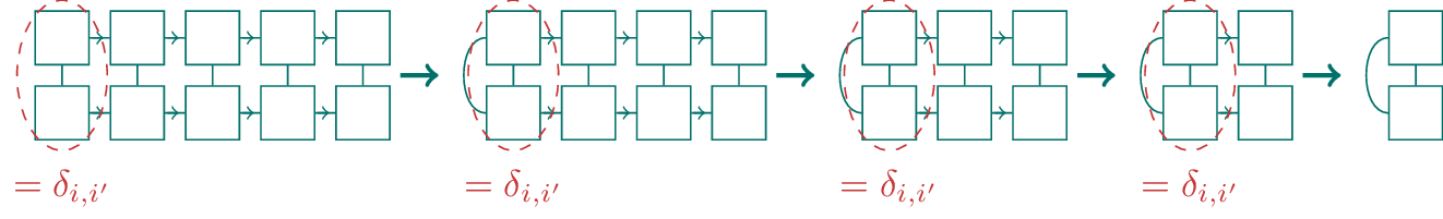
and an MPS with this property is said to be in left-canonical form. When the procedure of sequential SVDs from above is applied in reverse order, one equivalently obtains a right-canonical MPS.

An MPS can also be brought into mixed-canonical form. Starting with an MPS in left-canonical form, we can perform an SVD of the tensor at the end, which is not an orthogonal matrix. In graphical notation,

Thereby, we have generated an MPS in mixed-canonical form with the orthogonality center at position \(L-1\). The orthogonality center could also be shifted further to the left by applying additional SVDs.

1.4.2 Matrix product operators

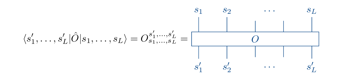
In analogy to the graphical representation of the wave function as a tensor with \(L\) legs, we can denote an operator \(\hat O\) acting on the wave function as a tensor with \(2L\) legs:

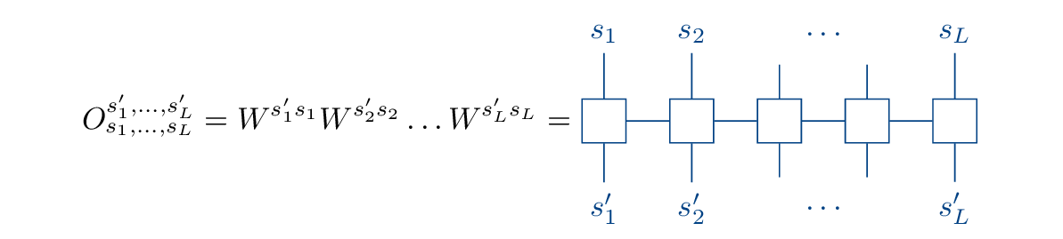
In analogy to the MPS, any operator can be brought into matrix product operator (MPO) form by means of the SVD,

and expectation values of the operator correspond to contractions of the form

The construction of some “simple” operators is rather obvious, namely those that are just products of single-site operators. Consider, for example, the two-point correlator of a spin-1/2 system, \[\begin{aligned} \hat\sigma_i^x\hat\sigma_j^z \equiv \mathbb 1_1\otimes\ldots\otimes \mathbb 1_{i-1}\otimes\hat\sigma_i^x\otimes\mathbb 1_{i+1} \otimes\ldots\otimes \mathbb 1_{j-1}\otimes\hat\sigma_j^z\otimes\mathbb 1_{j+1} \otimes\ldots\otimes\mathbb 1_L \end{aligned}\qquad{(37)}\] Defining the local tensors

we can write this operator diagrammatically as

or, equivalently, as

with the dimensions of all internal bond indices equal to one.

The construction of large sums of tensor product operators, e.g., the transverse-field Ising Hamiltonian 8, seems a much more daunting task. However, it turns out that there is a straightforward recipe to obtain the corresponding MPO. For this purpose, it is again useful to include explicitly the full tensor products of operators when writing the Hamiltonian, \[\begin{aligned} \hat H&=(-\hat S_1^z)\otimes\hat S_{2}^z\otimes\mathbb 1_3\otimes\mathbb 1_4\otimes\ldots +\mathbb 1_1\otimes (-\hat S_2^z)\otimes\hat S_{3}^z\otimes\mathbb 1_4\otimes\ldots +\ldots\nonumber\\ &\quad +(-g\hat S_1^x)\otimes\mathbb 1_2\otimes\mathbb 1_3\otimes\ldots +\mathbb 1_1\otimes(-g\hat S_2^x)\otimes\mathbb 1_3\otimes\ldots +\ldots \end{aligned}\qquad{(38)}\] The generation of the appearing operator strings can be viewed as the outcome of the execution of a finite-state machine (FSM). In this picture, each bond corresponds to a transition of the FSM. Reading the operator strings from right to left, there are three distinct states: (1) only \(\mathbb 1\) operators to the right of the current bond, (2) \(\hat S^z\) just right of the current bond, (3) a full interaction term or a transverse field term somewhere to the right of the current bond. The transitions between the states occur by adding specific operators to the next position: \(1\to1\) by \(\mathbb 1\), \(1\to2\) by \(\hat S^z\), \(1\to3\) by \(-g\hat S^x\), \(2\to3\) by \(-\hat S^z\), and \(3\to3\) by \(\mathbb 1\). These rules lead to a transition matrix at site \(i\) \[\begin{aligned} W^{(i)}= \begin{pmatrix} \mathbb 1 & 0 & 0 \\ \hat S^z & 0 & 0 \\ -g\hat S^x & -\hat S^z & \mathbb 1 \end{pmatrix}\ . \end{aligned}\qquad{(39)}\] Finally, the FSM has to start in state 1 and it must end in state 3, meaning that the first and the last transition matrices read \[\begin{aligned} W^{(1)}= \begin{pmatrix} -g\hat S^x & -\hat S^z & \mathbb 1 \end{pmatrix} \quad\text{and}\quad W^{(L)}= \begin{pmatrix} \mathbb 1 \\ \hat S^z \\ -g\hat S^x \end{pmatrix}\ . \end{aligned}\qquad{(40)}\] Expanding the product \(W^{(1)}W^{(2)}\ldots W^{(L)}\) yields exactly the sum of operator strings in Eq. 38. Inserting the explicit operator representations in the transition matrices yields exactly the MPO tensors \(W_{a_ia_{i+1}}^{s_i's_i}\) such that \[\begin{aligned} \hat H_{\text{TFIM}}=\sum_{\mathbf s,\mathbf s'}\sum_{a_1\ldots a_{L-1}}W_{a_ia_{i+1}}^{s_i's_i}|{\mathbf s'}\rangle\langle{\mathbf s}|\ . \end{aligned}\qquad{(41)}\]

1.4.3 Entanglement

1.4.3.1 Entanglement entropy

For a bipartite quantum system with Hilbert space \(\mathcal H=\mathcal H_A\otimes\mathcal H_B\) the von Neumann entropy of entanglement for a given state \(|{\psi}\rangle\in\mathcal H\) is defined as \[\begin{aligned} S_{A}^{\text{vN}}=-\text{tr}\big(\rho_A\ln\rho_A\big)\ . \end{aligned}\qquad{(42)}\] In this expression, \[\begin{aligned} \rho_A=\text{tr}_B\big(\rho\big)=\sum_{i,j,k}\psi_{i,k}\psi_{j,k}^*|{i_A}\rangle\langle{j_A}| \end{aligned}\qquad{(43)}\] denotes the reduced density matrix of subsystem \(A\) that is obtained by taking the partial trace \(\text{tr}_B(\cdot)\) of the density matrix \(\rho=|{\psi}\rangle\langle{\psi}|\) associated with the given state.

The reduced density matrix is a quantum generalization of a marginal probability distribution. \(\rho_A\) contains the complete information to describe all possible observations if measurements can only be performed on subsystem \(A\). The entanglement entropy is an information theoretic measure of correlations between both parts of the bipartition. It tells us how much we can learn about the state of the degrees of freedom in \(B\) by performing measurements on \(A\).

1.4.3.2 Schmidt decomposition

Let us denote a choice of orthonormal basis states of \(\mathcal H_A\) and \(\mathcal H_B\) by \(\{|{i}\rangle_A\}\) and \(\{|{j}\rangle_B\}\), respectively. Then, a general wave function of the composite Hilbert space can be written as \[\begin{aligned} |{\psi}\rangle=\sum_{i,j}\psi_{i,j}|{i}\rangle_A\otimes|{j}\rangle_B\ . \end{aligned}\qquad{(44)}\] Now, we can perform an SVD of \(\psi_{i,j}\), yielding \[\begin{aligned} |{\psi}\rangle=\sum_{i,j}\sum_{a=1}^{r}U_{i,a}S_{aa}V_{a,j}^*|{i}\rangle_A\otimes|{j}\rangle_B\ . \end{aligned}\qquad{(45)}\] with \(r=\text{min}\big(\text{dim}(\mathcal H_A),\text{dim}(\mathcal H_B)\big)\) and this expression can be further reorganized as \[\begin{aligned} |{\psi}\rangle&=\sum_{a=1}^{r}S_{aa}\Big(\sum_iU_{i,a}|{i}\rangle_A\Big)\otimes\Big(\sum_jV_{a,j}^*|{j}\rangle_B\Big) \nonumber\\ &=\sum_{a=1}^{r}S_{aa}|{a}\rangle_A\otimes|{a}\rangle_B\ . \end{aligned}\qquad{(46)}\] Here, \(\{|{a}\rangle_A\}\) and \(\{|{a}\rangle_B\}\) are sets of pairwise orthonormal vectors due to the orthonormality properties of \(U\) and \(V^\dagger\) and they can be extended to orthonormal bases of the respective subsystem. If we restrict the sum to run only over the \(\chi\leq r\) non-zero singular values, we obtain the Schmidt decomposition of \(|{\psi}\rangle\), \[\begin{aligned} |{\psi}\rangle&=\sum_{a=1}^{\chi}S_{aa}|{a}\rangle_A\otimes|{a}\rangle_B\ . \end{aligned}\qquad{(47)}\] Based on this, we immediately obtain the reduced density matrix in diagonal form, \[\begin{aligned} \rho_A=\sum_{a=1}^\chi S_{aa}^2|{a}\rangle_{A}{}_{A}{\langle{a}|} \end{aligned}\qquad{(48)}\] and, thereby, the von Neumann entropy of entanglement \[\begin{aligned} S_{A}^{\text{vN}}=-\sum_{a=1}^{\chi}S_{aa}^2\ln s_a^2\ . \end{aligned}\qquad{(49)}\] Due to the normalization of \(|{\psi}\rangle\) we furthermore know that \(\langle{\psi|\psi}\rangle=\sum_aS_{aa}^2=1\). Hence, we can read off that \(S_{A}^{\text{vN}}=0\) in the case of a single non-vanishing singular value and \(S_{A}^{\text{vN}}=\ln\chi\) if \(S_{aa}^2=\frac1\chi\ \forall a\). These are the extreme cases of minimal and maximal entanglement (with the absolute maximum given by \(S_{A}^{\text{vN}}=\ln(r)\)). Correspondingly, if we consider the MPS constructed in Section 1.4.1, we learn from the Schmidt decomposition that the magnitude of the bond dimensions \(\chi_i\) directly corresponds to the amount of entanglement that can be captured within the representation. MPS allow us to write weakly entangled wave functions in a compressed form.

1.4.3.3 Scaling laws of entanglement entropy

A quantum state \(|{\psi}\rangle\) is said to satisfy an area law of entanglement if for any bipartition into parts \(A\) and \(B\) the corresponding entanglement entropy is proportial to the area of the boundary \(\partial A\), \[\begin{aligned} S_A^{\text{vN}}\propto\partial A\ . \end{aligned}\qquad{(50)}\] By contrast, the maximum possible entanglement entropy grows proportionally with the number of degrees of freedom within \(A\), i.e., with the volume of \(A\). As part of the numerical experiments that you will perform in this project you will find that random states typically exhibit this behavior.

Remarkably, however, the ground states of gapped one-dimensional Hamiltonians of spin systems with local interactions are known to satisfy an area law of entanglement  [3]. In particular, the surface that separates two subsystems in a one-dimensional chain does not grow with the subsystem size. Hence, the entanglement entropy of gapped one-dimensional ground states is a constant.

Clearly, this statement does not apply at the critical point of a quantum phase transition, where the excitation energy gap vanishes. In one-dimensional systems the entanglement entropy of a subsystem of size \(l\) acquires a logarithmic correction to the area law and takes the form \[\begin{aligned} S^{\text{vN}}(l)=\frac{c}{6}\ln\bigg(\frac{2L}{\pi a}\sin\Big(\frac{\pi l}{L}\Big)\bigg)+\mathcal O(1)\ . \end{aligned}\qquad{(51)}\] This functional form can be derived, because the scale-invariance of the system at the critical point admits an effective description in terms of a conformal field theory (CFT), which is analytically tractable  [4]. In the expression above \(c\) denotes the central charge that characterizes the CFT, \(L\) is the system size, and \(a\) is the ultraviolet cutoff, i.e., the lattice spacing. Eq. 51 translates into a logarithmic scaling of the half-chain entanglement entropy with system size by considering \(l=L/2\): \[\begin{aligned} S_{|A|=\frac L2}^{\text{vN}}=\frac{c}{6}\ln L+\mathcal O(1) \end{aligned}\qquad{(52)}\]

In this project you will exploit the straightforward access to entanglement entropy within the MPS framework to test the CFT predictions for microscopic model Hamiltonians.

1.4.4 Density Matrix Renormalization Group

For a gentler introduction, we again refer to a video from the Computation Many-Body Physics lecture:

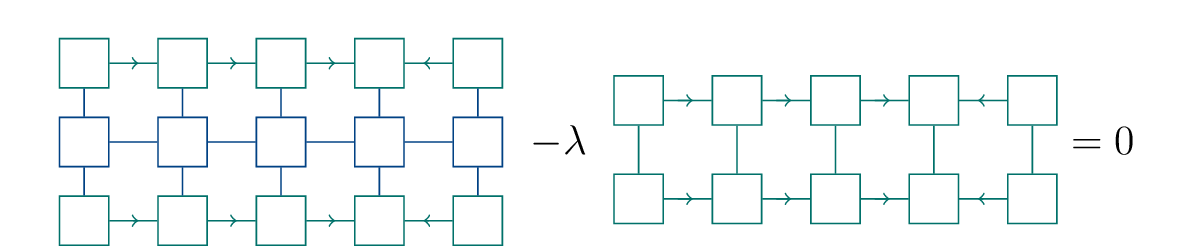
Having introduced the MPS representation of many-body wave functions, we now turn to an algorithm that makes extensive use of the MPS structure to find lowest-energy states of one-dimensional quantum systems. The starting point is a many-body Hamiltonian \(\hat H\) that describes the system of interest. The objective is to find the MPS \(|{\psi}\rangle\) that minimizes the total energy expectation value \[\begin{aligned} E=\frac{\langle{\psi|\hat H|\psi}\rangle}{\langle{\psi|\psi}\rangle}\ . \end{aligned}\qquad{(53)}\] To account for the normalization one can introduce a Lagrange multiplier \(\lambda\) and optimize the constrained problem \[\begin{aligned} \langle{\psi|\hat H|\psi}\rangle-\lambda\langle{\psi|\psi}\rangle\ , \end{aligned}\qquad{(54)}\] or, pictorially,

The idea of the Density Matrix Renormalization Group (DMRG) algorithm is now, that this optimization can be performed based on the MPS structure iteratively, one tensor at a time. An individual DMRG step consists of solving \[\begin{aligned} \frac{\partial}{\partial A_{a_{l-1},s_l,a_l}}\big(\langle{\psi|\hat H|\psi}\rangle-\lambda\langle{\psi|\psi}\rangle\big)=0\ , \end{aligned}\qquad{(55)}\] where \(A_{a_{l-1},s_l,a_l}\) is one of the tensors in the MPS. As the MPS is linear in each of the tensors, taking the derivative with respect to the entries of one tensor simply means removing the tensor in our graphical representation. Hence, the equation to solve is

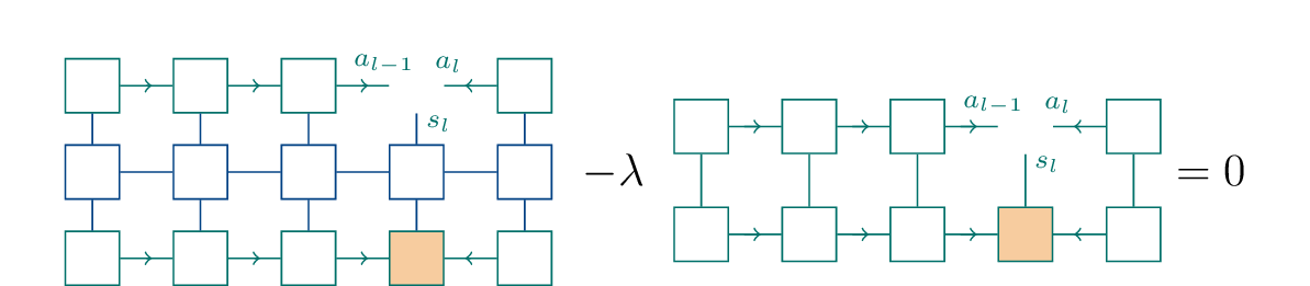
In the notation above we already assumed implicitly that the MPS is in mixed-canonical form with the orthogonality center at the position of the tensor that we are targeting. This means that we can easily perform the contraction of the second term and are left with

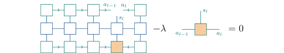
By summarizing the triple index into a composite index \((a_{l-1},s_l,a_l)\), we arrive at an eigenvalue problem \[\begin{aligned} Hv-\lambda v=0\ . \end{aligned}\qquad{(56)}\] As we are after the lowest energy MPS, we need to solve this eigenvalue problem for the eigenvector \(v_0\) with the smallest eigenvalue \(\lambda_0\); in fact, given the solution \(v_0\), \(\lambda=v_0^\dagger Hv_0\) is our current guess for the optimal energy.

With this local optimization procedure at its core, the full DMRG algorithm consists of sweeps through the MPS. Starting with an MPS in right-canonical form, the tensor at the orthogonality center is optimized by solving the eigenvalue problem above. Then, the orthogonality center is moved to the neighboring tensor by means of an SVD on order to optimize this tensor. This procedure is continued until the other end of the MPS is reached, thereby completing the right sweep. Next, one performs a left sweep, where the tensors are updated sequentially in the reverse order. This sweeping is continued until convergence.

2 Preparation

2.1 Theory

While you familiarize yourself with the theoretical background, find answers to the following questions:

1. What is the MPO form of the string correlator defined in Eq. 24?

2. Can you write the individual steps of the DMRG algorithm (including the shifting of the orthogonality center) in the diagrammatic language?

2.2 Coding

For this project you will use the ITensors.jl library  [5] that provides an implementation of core functionality and basic tensor network algorithms in julia. As preparation, ensure that the library runs on the computer you will use for the project. Moreover, read the sections “Perform a basic DMRG calculation” and “Compute excited states with DMRG” of the DMRG example https://itensor.github.io/ITensors.jl/stable/examples/DMRG.html and use the documentation to find out how to compute operator expectation values and entanglement entropy of a given MPS.

Central points to understand when studying the documentation are

• Which parameters control the accuracy of the DMRG simulation? How do you pass them to the dmrg routine?

• How can you compose a custom Hamiltonian MPO?

• How can you compose the MPO for the string correlator defined in 24?

• How can you multiply MPOs with MPSs? How can you compute expectation values of MPOs?

3 Tasks

3.1 Warmup: Decomposition into a Matrix Product State

For \(L\) spin-1/2 degrees of freedom, generate a random state vector in the form of a big tensor with \(L\) 2-dimensional external indices. Then follow the prescription for an iterative decomposition of the big tensor into a product of one tensor per site using successive SVDs as described in Section 1.4.1.

1. Plot the entanglement entropy for each possible cut of the MPS (averaged over a few realizations). What do you observe?

2. Plot the entanglement spectrum (i.e. the singular values) for the bipartition at the center of the chain. Is the random state compressible?

Hints for the implementation using ITensors.jl:

• Generate random tensors using the randomITensor function.

• ITensors.jl implements an interface for the SVD of ITensor objects in their svd function.

• The commoninds function returns the index (or indices) shared by two tensors.

3.2 Transverse-field Ising model

1. Verify the existence of a long range ordered phase in the transverse field Ising model by computing the squared magnetization \(\langle{\hat M_z^2}\rangle\) across a range of values of the transverse field.

2. Determine the value \(g_c\) that separates the two phases of the transverse-field Ising model. For this purpose it is useful to resort to the Binder cumulant of the order parameter, \[\begin{aligned} U_L=1-\frac{\langle{\hat M_z^4}\rangle_L}{3\langle{\hat M_z^2}\rangle_L^2} \end{aligned}\qquad{(57)}\] For different (large enough) values of \(L\) this quantity exhibits a unique crossing point as a function of \(g\) at \(g_c\). Therefore, its is particularly useful to read of the critical value.

3. The finite size scaling form of the Binder cumulant is \[\begin{aligned} U_L(\epsilon)=F_U(\epsilon/L^{-1/\nu}) \end{aligned}\qquad{(58)}\] Determine the value of the critical exponent \(\nu\) by performing a scaling collapse of the Binder cumulant.

4. The dmrg routine ITensors.jl library easily allows to constrain the ground state search to the subspace orthogonal to a set of given reference wave functions. Thereby, after having found a ground state \(|{\psi_0}\rangle\) you can then look for the next excited state \(|{\psi_1}\rangle\), which is the lowest energy state orthogonal to \(|{\psi_0}\rangle\). Use this to compute the excitation energy gap \(\Delta E\) as a function of the transverse field. Can you confirm that this gap closes at the critical point? Use your previously determined value of \(\nu\) to determine the dynamical critical exponent \(z\) via the finite size scaling form given in Eq. 7.

5. By computing the half-chain entanglement entropy of the ground state at the critical point for a range of system sizes, determine the central charge by probing the scaling relation Eq. 52. Can you also confirm Eq. 51?

3.3 Bilinear-biquadratic spin-1 chain

1. Implement the bilinear-biquadratic Hamiltonian and compute the ground state at the AKLT point. Does it exhibit the expected features?

2. Determine the critical point \(\theta_c\) with \(\sin(\theta_c)<0\) that separates the phase containing the AKLT point from its neighboring phase by examining the asymptotic value of the string order parameter 24 at large distances \(|i-j|\).

3. Determine the central charge at \(\theta_c\).
   Hint: There are two ways to probe the scaling relation, where finding the ground state at different system sizes is more straightforward, but also computationally expensive. Can you find a way which also works with a single ground state? If you observe any undesirable effects, how can you work around them?

References

---

1. To be a bit more concrete: If we consider a system, where the phase transition occurs by tuning an external control parameter \(g\) across a critical value \(g_c\), then the dimensionless measure of distance to the critical point can be defined as \(\epsilon=(g-g_c)/g_c\).↩︎

Materials

• Instruction PDF