Traffic flow modelling

[deutsche Version]

Cellular automata (CA) are models that are discrete in space, time and state variables. The latter property distinguishes CA e.g. from discretised differential equations. Due to the discreteness, CA are extremely efficient in implementations on a computer.

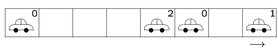
To describe the state of a street using a CA, the street is first divided into cells of length 7.5 m. This corresponds to the typical space (carlength + distance to the preceding car) occupied by a car in a dense jam. Each cell can now either be empty or occupied by exactly one car. Each vehicle is characterized by its current velocity v which can take the values v=0,1,2,... ,v_max. Here v_max corresponds e.g. to a speed limit and is therefore the same for all cars (in the simplest case). A typical configuration of the road is shown in the following figure.

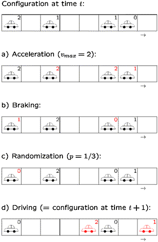
Now one needs to specify rules that define the temporal evolution of a given state. The simplest rule set, which leads to a realistic behaviour, has been introduced in 1992 by Nagel und Schreckenberg [3]. It consists of 4 steps that have to applied at the same time to all the cars (parallel or synchronous dynamics).

Step 1: acceleration All cars that have not already reached the maximal velocity vmax acceleration by one unit: v -> v+1 Step: safety distance If a car has d empty cells in front of it and is its velocity v (after step 1) larger then d, then it reduces the velocity to d: v -> min{d,v} Step 3: randomization With probability p, the velocity is reduced by one unit (if v after step 2):v -> v-1 Schritt 4: driving After steps 1-3 the new velocity vn for each car n has been determined forward by vn cells: xn -> xn+vn. The figure on the right shows for a specific example, how a configuration at time t+1 is updated step-by-step to obtain the new configuration at time t.

What is the interpretiuon of those rules? Step 1 describes the desire of the drivers to drive as fast as possible (or allowed). Step 2 encodes the interaction between the cars. In this simple model, interactions only occur to avoid accidents. Step 3, in a very simple way, corresponds to many complex effects that play an important role in real traffic. E.g. a single car will usually not move with a constant speed, but there are always small fluctuations of the velocity. An important point are overreactions at braking. A car that had to brake in step 2 will, with some probability p, brake even further than neccessary to avoid a crash. This kind of imperfect driving can lead to a chain reaction, if the density of vehicles is large enough. In the end it might lead to a car that has to stop and so leads to the creation of a jam. This jams occurs without obvious external reason and is therefore called ``jam out of nowhere'', ``phantom jam'' or spontaneous jam. It shows the extreme importance of step 3, which reflects the imperfect behaviour of the drivers. Finally, in step 4, all cars move according to their new velocity.

The above rule set is minimal in the sense that leaving out one of the 4 steps no longer leads to a realistic behaviour. Here realistic behaviour means that spontaneous jamming occurs and the so-called fundamental diagram, i.e. the relation between flow and density, is reproduced correctly. For small densities the flow is proportional to the density because there is almost no interaction between the cars. Then they drive with their desired velocity v_max (up to fluctuations). At higher densities the interaction becomes important and deviations from the linear behaviour can be observed. Finally the interactions start to dominate and the flow decreases with increasing density.

The dynamics can be visualized nicely by the Java-Applet. In the lower left corner the positions of the vecicles on a ring with periodic boundary conditions (i.e. the cars move in circles) are displayed. Above the ring the trajectories of the vehicles are shown. The left boundary (blue line) corresponds to the blue line (at 3 o'clock) on the ring. The velocity are symbolized by different colours. The momentary velocity distribution is shown at bottom in the middle diagram. The other diagram shows the momentary distribution of the gaps to the next car ahead. The other three diagrams on the right side are different versions of the fundamental diagram. The top graph shows the current as function of density. This is the classical form of the fundamental diagram. Below the average velocity is shown in dependence of the density or the flow, respectively. All three versions of the fundamental diagram are equivalent since the three quantities density r, flow J and average velocity v are not independent, but related through the hydrodynamical relation J=r v. It should be mentioned that all quantities in the diagrams are measured locally, i.e. by averaging only over a part of the ring. Therefore the (local) density can take different values also the total number of cars (and thus the global density) is fixed.

The simulation show the typical spontaneous jams (red). One also can observe the typical stop-and-go behaviour where a car shortly after leaving one jam has to stop due to the next jam. The global density can be changed using the controller ``global density''. Clearly the number of jams changes. It is also interesting to change the randomization parameter p über ``Slowdown prob. p'' for fixed density. Note that for p=0 a completely different behaviour occurs.

The applet allows also to study a different variant of the Nagel-Schreckenberg model. Clicking the button ``NaSch'' one can change to ``VDR''. VDR is the abbreviation of ``velocity-dependent randomization'' and denotes the important difference to the NaSch model. In the latter the randomization parameter p is constant. In the VDR model [4], on the other hand, p depends on the velocity of the vehicle after the last time step. For standing cars a larger value p₂ is chosen than for that p for moving cars. The only difference between the VDR model and the NaSch model is therefore only an additional step in the update procedure:

Step 0: determination of the randomization parameter p(v) For standing cars (v=0) one has p(v=0)=p2 . For moving cars ,(v>0) the randomization is chosen as p(v)=p.

This step has to be carried out before the NaSch steps 1-4. All other update steps are unchanged. p₂ can be controlled by the button ``Slowdown prob. of stopped cars p2''.

To see the difference between the behaviours of the NaSch and the VDR models clearly, choose a small value of p, e.g. p=0.01 and a rather large value for p₂, e.g. p₂=0.5. One can can clearly see that (for densities not too small) that after some time a phase-separated state evolves that consists of a large jam and a free-flow region.

Literature:

[1]	D. Chowdhury, L. Santen and A. Schadschneider: Statistical physics of vehicular traffic and some related systems , Physics Reports 329, 199 (2000)
[2]	S. Wolfram, Theory and Applications of Cellular Automata, (World Scientific, 1986)
[3]	K. Nagel and M. Schreckenberg, A cellular automaton model for freeway traffic, J. Physique I 2, 2221 (1992)
[4]	R. Barlovic, L. Santen, A. Schadschneider and M. Schreckenberg, Metastable states in cellular automata for traffic flow, Eur. Phys. J. B 5, 793 (1998)