| Model Definition |
| Introduction |
|
Methods from physics have been successfully used for the investigation
of vehicular traffic for a long time. On the other hand, pedestrian dynamics has not been studied as extensively. Due to its generically two-dimensional nature, pedestrian motion is more difficult to describe in terms of simple models. However, many interesting collective effects and self-organization phenomena have been observed: 1.) Jamming: At large densities various kinds of jamming phenomena occur, e.g. when many people try to leave a large room at the same time. This clogging effect is typical for a bottleneck situation. Other types of jamming occur in the case of counterflow where two groups of pedestrians mutually block each other. This happens typically at high densities and when it is not possible to turn around and move back, e.g. when the flow of people is large. 2.) Lane formation: In counterflow, i.e. two groups of people moving in opposite directions, a kind of spontaneous symmetry breaking occurs. The motion of the pedestrians can self-organize in such a way that (dynamically varying) lanes are formed where people move in just one direction. In this way, strong interactions with oncoming pedestrians are reduced and a higher walking speed is possible. 2.) Oscillations: In counterflow at bottlenecks, e.g. doors, one can observe oscillatory changes of the direction of motion. Once a pedestrian is able to pass the bottleneck it becomes easier for others to follow him in the same direction until somebody is able to pass (e.g. through a fluctuation) the bottleneck in the opposite direction. 3.) Patterns at intersections: At intersections various collective patterns of motion can be formed. A typical example are short-lived roundabouts which make the motion more efficient. Even if these are connected with small detours the formation of these patterns can be favourable since they allow for a ''smoother'' motion. 4.) Trail formation: In counterflow, i.e. two groups of people moving in opposite directions, a kind of spontaneous symmetry breaking occurs. The motion of the pedestrians can self-organize in such a way that (dynamically varying) lanes are formed where people move in just one direction. In this way, strong interactions with oncoming pedestrians are reduced and a higher walking speed is possible. 4.) Emergency situations: In emergency situations many counter-intuitive phenomena (e.g. ''faster-is-slower'' and ''freezing-by-heating'' effects) can occur. We have introduced a new kind of CA model which -- despite its simplicity -- is able to reproduce the observed collective effects. This is essential if one intends to use the model for real applications, e.g. the optimization of evacuation procedures. The model takes its inspiration from the process of chemotaxis. Some insects create a chemical trace to guide other individuals to food places. This is also the central idea of the active-walker models used for the simulation of trail formation. In our approach the pedestrians also create a trace. In contrast to trail formation and chemotaxis, however, this trace is only virtual although one could assume that it corresponds to some abstract representation of the path in the mind of the pedestrians. Its main purpose is to transform effects of long-ranged interactions (e.g. following people walking some distance ahead) into a local interaction (with the ''trace''). This allows for a much more efficient simulation on a computer. |
| Basic principles of the model |
|
In the model the space is discretized
into small cells which can either be empty or occupied by exactly one
pedestrian. Each of this pedestrians can move to one of its unoccupied
neighbour cells at each discrete time step t to t+1 according to
certain transition probabilities. The probabilities are given by the interaction with two floor fields. The two fields determine the transition probability in that way, that the particle movement is more likly in direction of higher fields. These two fields shall be regarded shortly in the following and the basic update rules of the model are summarized. The static floor field S: The static floor field S does not evolve with time and is not changed by the presence of the pedestrians. Such a field can be used to specify regions of space which are more attractive, e.g an emergency exit or shop windows. In case of the here considered evacuation processes, the static floor field describes the shortest distance to a an exit door, lying at the middle of the top wall of the room. The picture below shows graphical represantations of S for different geometries. 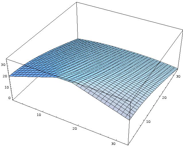
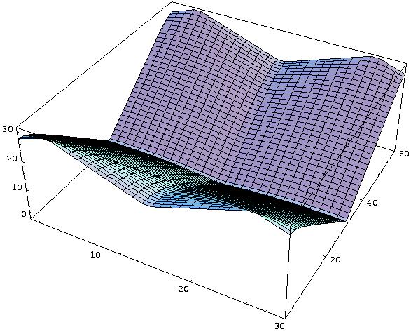
S is calculated due to a certain distance metric for each lattice site so that the field values are increased in the direction to the door. The field values are highest for the door cells. The dynamic floor field S: The dynamic floor field D is a virtual trace left by the pedestrians and has its own dynamics, i.e. diffusion and decay. It is used to model an attractive interaction between the particles. The picture below shows 3-dimensional plots of D for three stages during evacuation process. 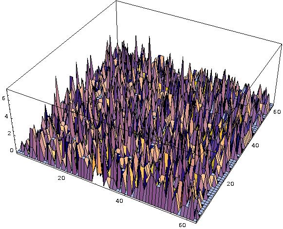
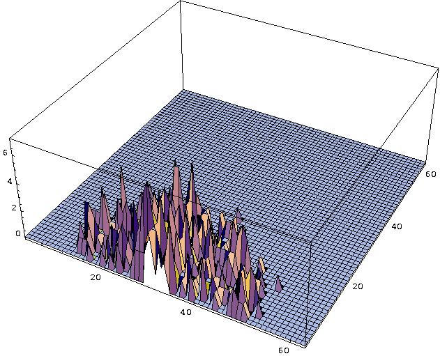
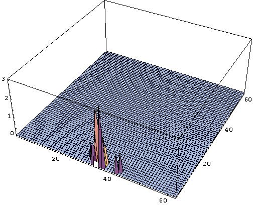
At t=0 for all sites (i,j) of the lattice the dynamic field is zero, i.e. D(i,j)=0. Whenever a particle jumps from site (i,j) to one of the neighbouring cells, D of the starting place is increased by one. Therefore D has only non negative integer values and can be compared to a bosonic field, i.e. the bosons dropped by the pedestrians during their movement create the virtual trace. Thus the field value D(i,j) corresponds to D(i,j) bosons. The dynamic floor field is time dependent, it has diffusion and decay controlled by two parameters alpha in [0,1] and delta in [0,1], which means broadening and dilution of the trace. In each time step of the simulation each single boson of the whole dynamic field D decays with the probability delta and diffuses with the probability alpha to one of its neighbouring cells. Finally this yields to D=D(t, delta, alpha ). Note that the dynamic floor field D is only altered by moving particles and therefore it corresponds more to a virtual velocity density field, then a particle density field. |
 Main page Main page | Parameters | Examples | Miscellaneous |